Introduction
Overview
Teaching: 10 min
Exercises: 0 minQuestions
Why are jupyter notebooks useful for cleaning and wrangling data?
Objectives
Describe how jupyter notebooks provide a method of documenting the steps invovlved in cleaning and wrangling data
Why should I care about this?
If you have ever worked with a set of data in an Excel spreadsheet, Google sheet or CSV file you have probably had to modify that data in some manner to use it. You probably have needed to add or remove columns and rows or do some summations or different arithmetic functions to the data. Excel and G-sheets work just fine for simple data. But what do you do when you have thousands and millions of rows of data? Or what if you have a bunch of the same type of dataset and your want to apply the same steps to each dataset or repeat this in the future? Manually doing this work doesn’t scale nor is what you did reproducible or easily shareable with others.
Jupyter notebooks provide a solution to this problem, allowing you to scale, automate, document, and reproduce parts of or your entire analysis. They also provide a method by which you can test newer sections of your analysis as you move from having some initial data to an analysis product.
Here you will learn the basics of utilizing jupyter notebooks by using Python and a library called Pandas (Link to Pandas Website). The Pandas library helps provide various bells and whistles for both cleaning and analyzing your data. However, since it is built on top of Python a basic understanding of the Python (Link to Python Website) programming language is required. Through these tools you will learn how to analyze a raw dataset by cleaning it up and formatting it so that it can be used for further analysis or other workflows.
What this lesson will not teach you
- How to write basic python code
- How to set up a notebook environment
- How to run other programming languages e.g. R in jupyter notebooks
Notebook Programming Languages
Jupyter notebooks can contain various programming languages with R or Julia being possibilities.
Lesson Structure
The structure for this lesson will require participants to run a jupyter notebook. In order to reduce the time required to get Jupyter notebooks setup and running we will be utilizing Binder (Link to Binder Website). Binder allows us to run a jupyter notebook using a predefined environment and github repository right from our browser. For this lesson we have already setup a binder notebook that links to the github repository for this lesson. There will also be link at the top of each episode to the Binder website for this lesson.
Link to Binder notebook for this Lesson
Key Points
Notebooks help connect the code for cleaning and wrangling data to the documentation explaining what is being done and why.
Jupyter Notebook Interface
Overview
Teaching: 10 min
Exercises: 0 minQuestions
How is the jupyter notebook interface setup
Objectives
Describe the basics of the jupyter notebook interface
Demonstrate the various basic cell types notebooks use
Demonstrate how notebooks deal with code blocks and the concept of restarting the kernel
Notebook Basics
The button above will take you to the associated binder website for this lesson. When you load up the binder webpage you should be presented with a site that looks something like the image below.
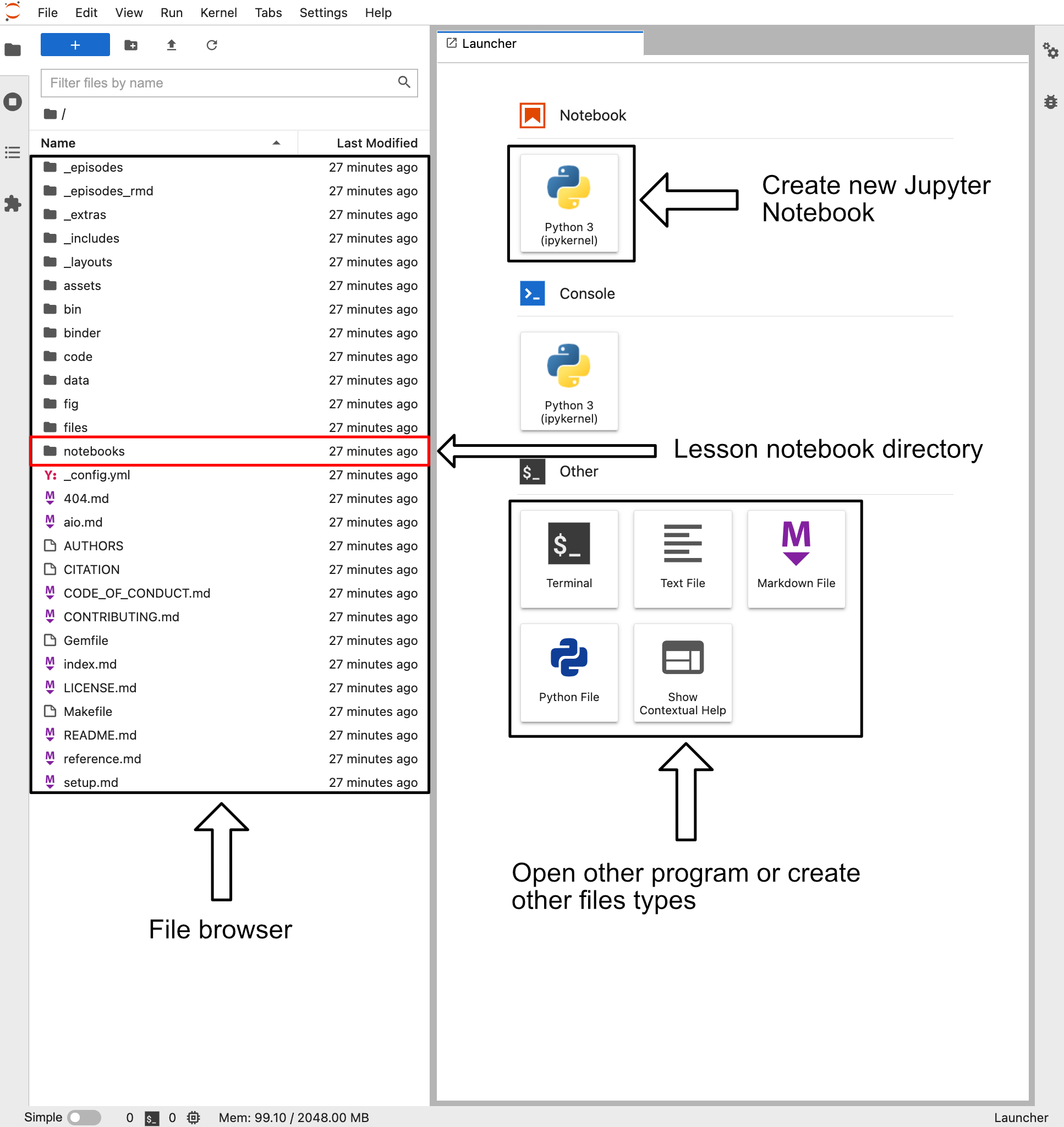
This site contains a variety of buttons to create various file types. However, for now we are going to do two things.
- Double click on the “notebook” directory in the file browser
- This directory contains all the Jupyter notebooks associated with this lesson
- Click on the “Python 3” box beneath the Notebook label. This button is next to the arrow labeled “Create new Jupyter Notebook”
- This will create a Jupyter notebook called “Untitled.ipynb” with a single blank cell
Once you click on on the Python 3 button under the notebook label you will be presented with a new screen which will look something like the image below (note that the image has been cropped to reduce space).

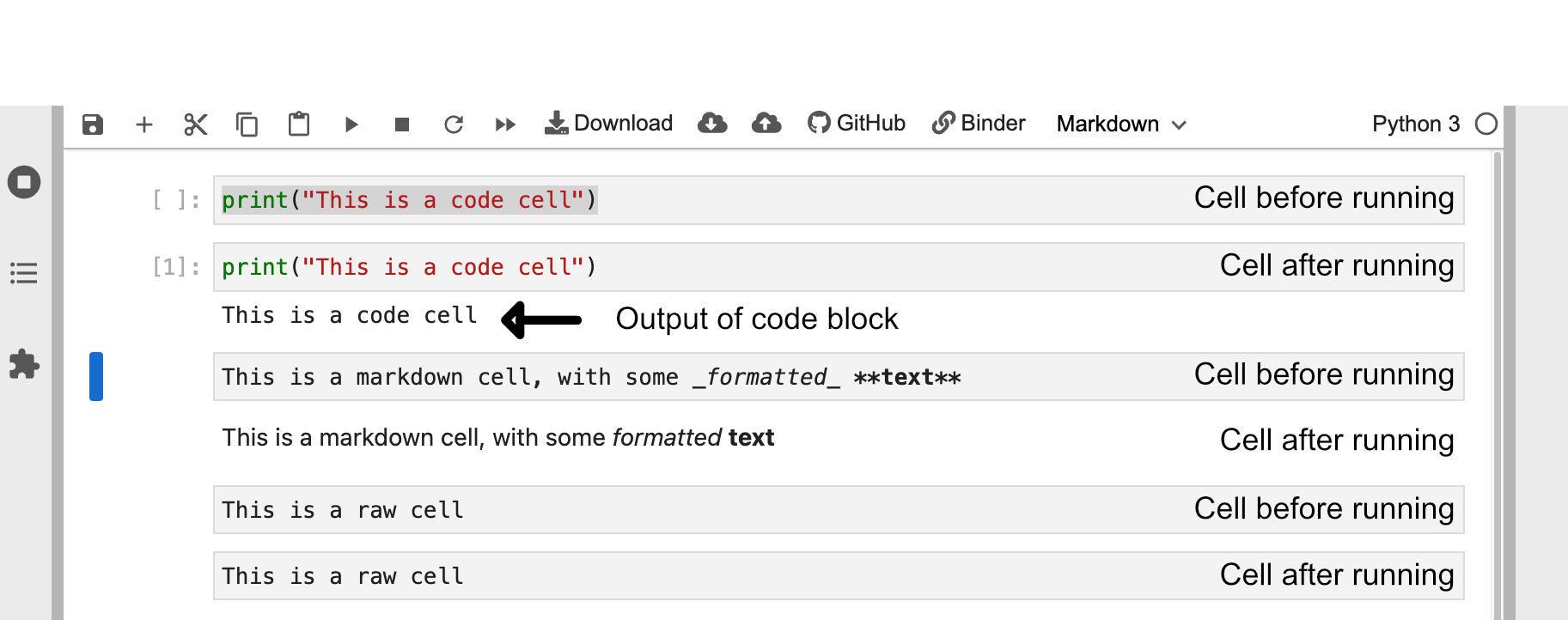
This notebook is blank except for a single cell. This blank cell is a code cell that you can type in. For example if you type in some python code like print("This is a code cell") and then click the run button you will see the output appear beneath the cell.
Cell Types
Cells are the base unit in Jupyter notebooks. A notebook is essentially just a collection of cells of different types. In Jupyter notebooks there are three primary types of cells:
- Code cells
- Code cells treat everything typed inside them as code
- When they are “run” they will run the code they find inside them
- Markdown cells
- Markdown cells treat everything typed inside them as markdown
- When they are “run” they will format the text inside them based on jupyter markdown
- Raw cells
- These cells treat everything inside them as raw text
- If you “run” these cells nothing will happen
If you double click the jupiter notebook called “02-jupyter-notebook-interface.ipynb” that can be found in the file browser side tab you will be presented with a notebook that already has some cells filled in. Underneath the header “Cell Types” you will find three different cells that each correspond to one type of cell. You can select the top cell and then click the run button three times to run all three cells of these cells.
Running Cells
You can also run a selected cell by pressing Shift+Return
You will see that the action performed after running a cell is different for each of the cells.
Editing Cells
You can also edit cells after running them by clicking on the cell like normal text. For markdown cells you will need to double click on the cell area in order revert it back into a editable format.
Markdown and raw cells can be edited and run repeatedly without much issue. However, when editing code blocks you have to be more careful. When you run a code cell you are running that piece of code. Even if you delete or edit the code block after running it the changes it made will remain until the Kernel is restarted.
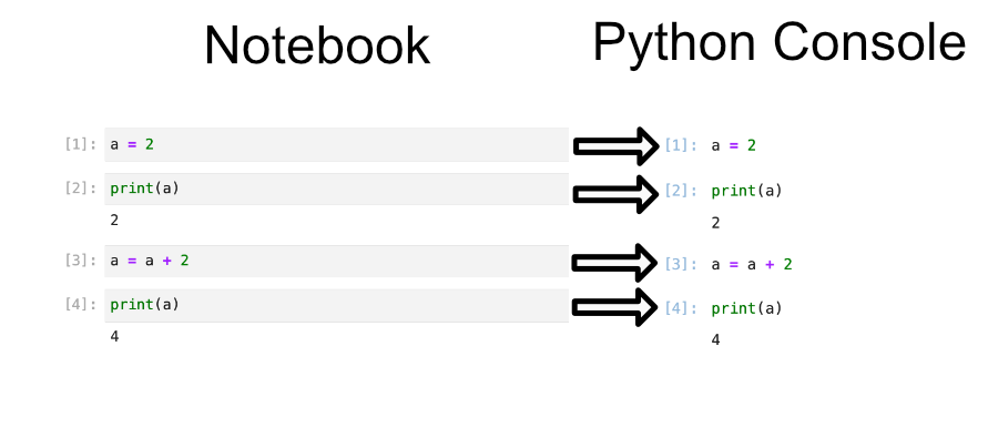
A good way to think about code cell execution in a notebook is that you are essentially copy pasting the code cell into a python console. The image below gives a visual example of this with the notebook cells on the left, and a python code that does the same set of commands on the right. You can try running the cells found in the left image by looking for the header “Editing Cells” in the Binder notebook “02-jupyter-notebook-interface.ipynb”.
To show the dangers of rerunning cells we can try rerunning the two bottom cells containing the code a = a + 2 and print(a). This will be reflected as a fifth and sixth command executed in the python console. You can see this reflected in the Python console below where the same commands have been issued in the same order. So despite the fact that we only have four cells of python we have executed 6 cells worth of code.
Rerunning Cells
Rerunning code cells will erase the output of that code cell and update the counter next to the cell with the most recent time the cell was run.
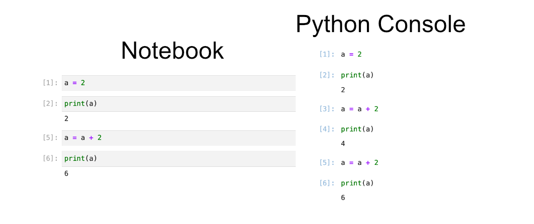
Rerunning code cells is not recommended since it obscures what the notebook’s code cells are doing and can make it very difficult for anyone reading your notebook to accurately rerun your analysis.
Jupyter Notebook Cheatsheet
The image below is a cheatsheet of some of the buttons not discussed in this episode that might be good to know for the future. Feel free to come back to it if you are confused later on.

Key Points
A jupyter notebook is divided into cells that are either code, markdown, or raw
Cells can be “run” leading to either the execution of code or formatting of markdown depending on the cell type
Code cells can be rerun, but this should be avoided to prevent obscuring the notebooks workflow
Loading and Handling Pandas Data
Overview
Teaching: 20 min
Exercises: 0 minQuestions
How are Pandas data structures setup?
How to load data into Pandas?
How to write data from Pandas to a file
Objectives
Understand the usefulness of Pandas when loading data
Understand how to load data and deal with common issues
Pandas Data Structures
For this episode you should follow along inside the Jupyter notebook associated with this episode. The jupyter notebooks for this entire lesson can be found in Binder (Link to lesson’s Binder website). You will have to navigate to the “notebook” directory in the file browser to find the notebook associated with this episode.
Before we start loading data into Pandas we need to become familiar with 2 of the primary data structures of Pandas:
- Series
- DataFrames
The reason we use Series and DataFrames rather than native python data structures to hold our data is because there are additional attributes and methods associated with Series and DataFrames that will be useful for wrangling and analytics. One of the primary benefits of Series and DataFrames over native python data structures is that it is a very natural way to describe a data set in an excel-like manner by referencing the rows and columns of our data with labels of our choosing.
Pandas Series Vs. DataFrames
Pandas has two principal data structures, Series and DataFrames. If you are familiar with Microsoft’s Excel application then you can liken Series to single columns (or rows) in an Excel sheet and DataFrames to entire tables (or spreadsheets).
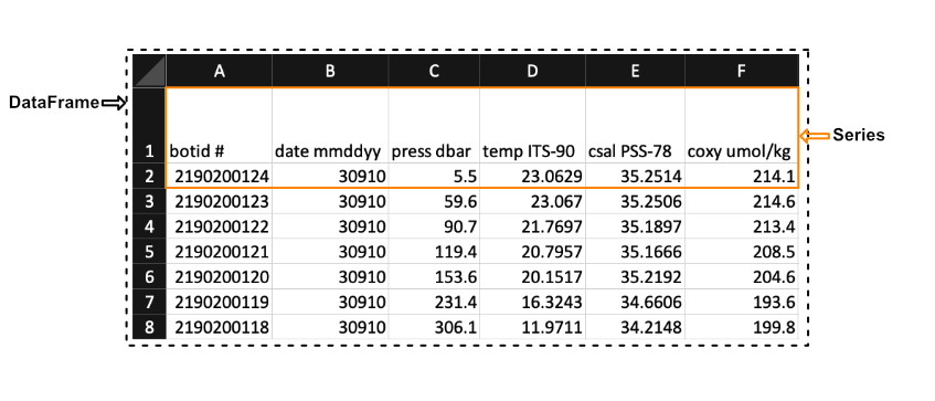
We see in the image above that a Series in the context of Excel could be the first row of the spreadsheet, while a DataFrames would be the entire spreadsheet. In other words, a DataFrames is simply a collection of labeled Series.
Pandas Data Types
When creating a Series Pandas will store all the data as the same type. The mapping from the native python types to what they would be in Pandas is summarized below.
| Python Type | Equivalent Pandas Type | Description |
|---|---|---|
string or mixed |
object |
Columns contain partially or completely made up from strings |
int |
int64 |
Columns with numeric (integer) values. The 64 here refers to size of the memory space allocated to this type |
float |
float64 |
Columns with floating points numbers (numbers with decimal points) |
bool |
bool |
True/False values |
datetime |
datetime |
Date and/or time values |
Pandas DataFrames Basics
DataFrames are essentially ordered collections of Series with two associated Index objects, one to label rows and another to label columns. Reiterating the example mentioned earlier, it helps to think of DataFrames as MS. Excel spreadsheets where each row (or column) as an individual Series.
You can create DataFrames from either loading in a file e.g. a csv file or by converting it from a native Python data structure. However, here we will be focusing on loading data from a file and turning it into a DataFrame.
Creating Pandas
SeriesYou can also create Pandas
Seriesfrom files or native python data structures (Link to more info).
Before we can load in data from a file we need to load the pandas package. Pandas is often imported alongside as pd to reduce the amount of characters needed to use the different methods within it.
import pandas as pd
Loading and Parsing Data
Pandas can load in data from a variety of file formats. However, in most cases you will be loading in data from a plain text file since this is one of the most common and simple ways to store data. Plain text files only contain text without any special formatting or code e.g. .txt, .csv, or .tsv files.
To store data in a plain text file you need a standard way of distinguishing the individual data entries. For example, suppose a file contained the following text:
,column1,column2,column3,
row1,a,b,c
row2,d,e,f
row3,g,h,i
A human would see the text above and may be able to discern the 3 columns and 3 rows and the individual data entries and see that the file contains a table that looks like the one below.
| column 1 | column 2 | column 3 | |
|---|---|---|---|
| row1 | a | b | c |
| row2 | d | e | f |
| row3 | g | h | i |
However, a computer would have no idea how to parse this without any direction; to a computer the text above is just one string of characters. To help the computer parse the text, we could tell it that each data entry is separated by a column and each row is separate by a new line. This way of organizing data is called a plain text file format.
Most of the plain text file formats fall into one of the following two categories: Delimited and Fixed Width
- Delimitted files are organized such that columns and rows are seperated by a certain character called a delimiter
- Fixed width files are those where each entry in a column has a fixed number of characters
We will focus on the delimited .csv file type. csv is an acronym which stands for ‘Comma Separated Values’ and informs us that the column entries are delimited by commas and the rows are delimited by a new line. So, the example we discussed in this cell conforms to the .csv format.
Included in the Pandas toolkit is a collection of parsing functions to read and build DataFrames from data that is stored in a variety of formats. The Pandas function which parses and builds a DataFrame from a generic delimited plain text file is read_csv(). To run read_csv() with the default settings we only need to provide 1 positional argument, the path to the file we want to read. If we wanted to read a file in the same directory as our notebook called p and put the data into a new Pandas DataFrame, df, we would type df = pd.read_csv(p).
However, parsing plain text files can become a complicated procedure. To aid in the process, Pandas provides a lot of optional parameters that may be set when calling the read_csv() function. To learn more, see the read_csv() documentation, which summarizes all of the parameters. We will be covering many of the most important parameters throughout the rest of this lesson.
By default read_csv() will separate data entries when it encounters a comma and will separate rows by new lines encoded by ‘\n’. If we wanted to change this behavior so that read_csv() separates by tabs (encoded with \t), then we can set the optional parameter sep = '\t'. For instance, if we wanted to read the data in the file ‘tsv_example.tsv’, which is a tab separated values file, and save the data in a Pandas DataFrame called df, then we would type:
df = pd.read_csv('data/tsv_example.tsv', sep='\t')
Though read_csv() can handle .tsv files, there is a specific parsing function for .tsv files: read_table(). The difference between read_table() and read_csv() is that the default behavior for the latter is to separate using commas instead of tabs \t. The read_table() documentation is available at this link.
To perform the same operation (that is reading the data in the file tsv_exampletsv and save the data in a Pandas DataFrame called df), we may use the read_table() function without having to define our delimiter, since the default parameters will correctly parse our file.
df = pd.read_table('data/tsv_example.tsv')
Both methods will lead to an equivalent DataFrame.
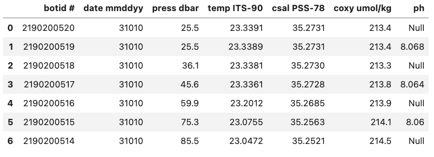
In the previous examples we loaded the entire dataset from the file we gave Pandas. However, when working with large datasets it is good practice to load your data in small pieces before loading the entire dataset to ensure that the file is parsed correctly. Small data sets are more manageable and errors are easier to spot, while large data sets take more time to parse. So, a good workflow is to read a small portion of the data and analyze the resulting data frame to see if you need to modify any of the default behaviors of the read function.
To load only up to a limited number of rows we can use the nrows parameter for both read_table() and read_csv(). For example, the file E3_tara_w1.csv is a csv file with over 200 rows, but if we wanted to read only the first 5 rows of this file we can call the Pandas read_csv() function and set nrows = 5:
df = pd.read_csv('data/tsv_example.tsv', nrows=5)
df.shape # Returns the number of rows and columns of the DataFrame 'df' (rows, columns)
(3, 7)
We see that the DataFrame df, that we saved the data in, has a shape attribute of (3, 7). This means that there are 3 rows (since we set nrows=3) and 7 columns (all the columns of the dataset).
Headers and Indexes
When we loaded the previous datasets read_csv() assumed that the first row in our .csv file contained headers for each of the columns. If we want to load in a dataset that does not contain a header row we can tell read_csv() that there is no header by setting header=None.
df = pd.read_csv("data/noheader_example.csv", header=None)
df
However, this does not mean that the DataFrame does not have headers but rather that Pandas will set them to be an integer value. An example is shown in the figure below:
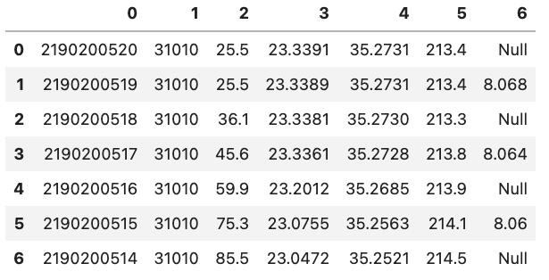
You might also notice that there is also a corresponding integer number in the far left side of each row. This is the index that is essentially the “name” for each row. If we have a column that is specifies each row in the input file we can tell Pandas to use that column instead of the default of using a integer. This can be done by e.g. setting index_col='unique_id' however, if you don’t have any headers you can also specify the column by using its integer location e.g. index_col=0. Note that the integer location of a column goes from left to right and starts at 0.
df = pd.read_csv('data/noheader_example.csv', header=None, index_col=0)
df
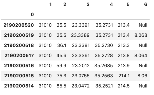
You can change the name of the index column by setting the index name attribute of the dataframe df.index.name = 'unique_id'.
Common Data Loading Problems
Though data storage in plain text files should follow certain formats like .csv for ‘Comma Separated Values’ and .tsv for ‘Tab Separated Values’, there is still some ambiguity on how things like missing entries, and comments should be denoted. For this reason Pandas has implemented functionality into the read_table() and read_csv() to help ‘clean’ plain text data.
Below we will go through two examples of common issues when loading in data.
Missing Values
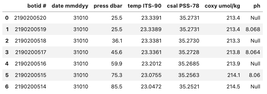
There are often missing values in a real-world data set. These missing entries may be identifiable in the dataset by a number of different tags, like ‘NA’, ‘N.A.’, ‘na’, ‘missing’, etc. It is important to properly identify missing values when creating a DataFrame since certain DataFrame methods rely on the missing values being accounted for. For example, the count() method of a DataFrame returns the number of non missing values in each column. If we want this to be an accurate count, then we need to be sure of pointing out all the tags which represent ‘missing’ to Pandas.
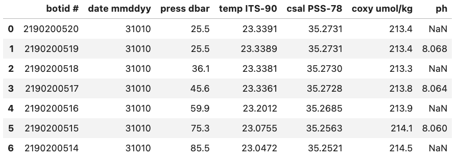
For example, if we were to load in a .csv where missing values are ‘Null’ and not specify this then Pandas will load these values in as objects. To let Pandas know that we want to interpret these values as missing values we can add na_values='Null'.
df = pd.read_csv("data/null_values_example.csv", na_values='Null')
df
Without na_values='Null':
With na_values='Null':
Auto NaN values
Pandas will interpret certain values as being NaN values even without user input. For example if ‘NULL’ is found then Pandas will treat it as a missing value and treat it as a NaN value.
Writing Data in Text Format
Now that we are familiar with the reading mechanisms that Pandas has implemented for us, writing DataFrames to text files follows naturally. Pandas DataFrames have a collection of to_<filetype> methods we can call; we will focus on to_csv(). to_csv() takes the parameter path (the name and location of the file you are writing) and will either create a new file or overwrite the existing file with the same name.
to_csv() has a number of optional parameters that you may find useful, all of which can be found in the Pandas documentation.
df.to_csv('data/new_file.csv')
Key Points
Pandas provides numerous attributes and methods that are useful for wrangling and analyzing data
Pandas contains numerous methods to help load/write data to/from files of different types
Wrangling DataFrames
Overview
Teaching: 20 min
Exercises: 0 minQuestions
How can you select individual columns or rows from a
DataFrame?How can you subset a
DataFrame?How can you sort a
DataFrame?Objectives
Learn how to select specific columns or rows from a
DataFrameLearn how to select rows based on conditions
Learn how to sort a
DataFrame’s rows or columns
Selection, Subsetting and Sorting a DataFrame
When exploring our data we will often want to focus our attention to specific rows, columns, and entries that satisfy certain conditions. We may want to either look at a single column of the data or work with a subset of the original data. This situation may occur because the source of your data was probably not using the information for the exact same purpose.
Furthermore, it is often helpful to sort our data set using a particular relation to identify patterns and to understand the data’s structure. For example, suppose the original data set we acquire and want to analyze describes a sport team’s performance for each game during a season and it is original ordered in chronological order. It may be interesting to sort the game play statistics using a different relation such as number of points scored to easily identify high and low scoring games.
As with previous episodes you should follow along in the notebook starting with ‘04’ that can be found at the following link Link to Binder.
Selection
Selecting data from a DataFrame is very easy and builds on concepts we discussed in the previous episode. As mentioned previously, in a DataFrame we have column names called headers and row names called indexes. Depending on how we loaded the data these might be integers or some other ID.
If we have the example DataFrame seen in the image below we can select and/or subset various combinations of rows and columns by using Pandas.
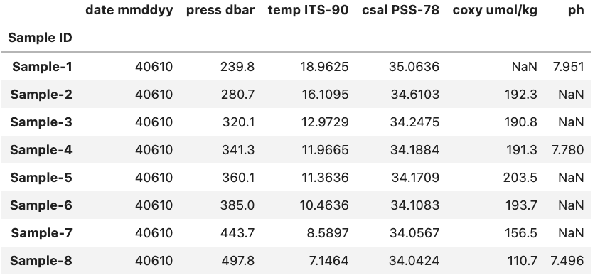
Selecting Columns
To start off lets focus on subsetting columns. If we have a DataFrame called df and a column called ‘ph’ we can subset the DataFrame using df['ph'].
df['ph']
Sample ID
Sample-1    7.951
Sample-2      NaN
Sample-3      NaN
Sample-4    7.780
Sample-5      NaN
Sample-6      NaN
Sample-7      NaN
Sample-8    7.496
Name: ph, dtype: float64
Selecting Rows
If on the other hand we want to access a subset rows we have to use a slightly different approach. While previously we could just pass the name of the column inside brackets if we want to access one or more rows we need to use the .loc or .iloc methods.
So if we again have a DataFrame called df and a row called ‘Sample-1’ we can access it using df.loc['Sample-1', df.columns].
df.loc['Sample-1', df.columns]
date mmddyy     40610.0000
press dbar        239.8000
temp ITS-90        18.9625
csal PSS-78        35.0636
coxy umol/kg           NaN
ph                  7.9510
Name: Sample-1, dtype: float64
The key difference between .loc and .iloc is that .loc relies on the names of the indexes and headers while .iloc relies instead on the index and header number. Here df.columns is providing the all the header names in the DataFrame called df and letting pandas know that we want a single row, but all of the header in the DataFrame.
If we were to use .iloc instead of .loc for the previous example and we know that ‘Sample-1’ is at index position 0 we would use df.iloc[0, :] and get the same result. You might notice that we also had to change df.columns to : when we used .iloc this is because df.columns provides the names of all the headers which is fine to do with .loc but not .iloc.
df.iloc[0, :]
date mmddyy     40610.0000
press dbar        239.8000
temp ITS-90        18.9625
csal PSS-78        35.0636
coxy umol/kg           NaN
ph                  7.9510
Name: Sample-1, dtype: float64
The
:operatorWhen used inside a bracket the
:operator will return the range between the two values it is given. For example if we had a python listxwith the following values [‘a’, ‘b’, ‘c’, ‘d’, ‘e’] and wanted to select ‘b’, ‘c’, and ‘d’ we can do this very concisely using the:operator.x = ['a', 'b', 'c', 'd', 'e'] x[2:5]With the output:
['b', 'c', 'd']
Selecting Columns and Rows Simultaneously
As we saw in the previous section we can select one or more rows and/or columns to view. For example if we wanted to view the ‘ph’ entry of ‘Sample-1’ from the previous example we could use .loc in the following manner.
df.loc['Sample-1', 'ph']
7.951
If we wanted to select multiple columns e.g. both the ‘ph’ and ‘Longitude’ columns we can change the code bit to fit our needs.
df.loc['Sample-1', ['ph', 'Longitude']]
temp ITS-90    18.9625
ph              7.9510
Name: Sample-1, dtype: float64
Using
.ilocYou can just as well use
.ilocfor the two examples above, but you will need to change the index and headers to their respective integer values i.e. the row number(s) and the header number(s).
Subsetting
Comparison operations (“<” , “>” , “==” , “>=” , “<=” , “!=”) can be applied to pandas Series and DataFrames in the same vectorized fashion as arithmetic operations except the returned object is a Series or DataFrame of booleans (either True or False).
Within a Single DataFrame
To start let focus on a single DataFrame to better understand how comparison operations work in Pandas. As an example lets say that we have a DataFrame like the one below stored in df:
If we wanted to identify which of the above samples come from a depth above 380 we start by finding column ‘press dbar’ using a less than condition of 380.
df['press dbar'] < 380
The output will be a Pandas Series containing a boolean value for each row in the df that looks like this.
Sample ID
Sample-1     True
Sample-2     True
Sample-3     True
Sample-4     True
Sample-5     True
Sample-6    False
Sample-7    False
Sample-8    False
Name: press dbar, dtype: bool
We can see that the first row and the last row are both True while the remaining rows are False and a quick look at the original data confirms that this is correct based on our condition. However, looking back at the original DataFrame is very tedious. If we instead want to view/save the rows that were found to have a depth < 380 we can either save the output Series to a variable and use that or directly place the previously used code within a bracket. Both methods are equivalent and shown below.
good_rows = df['press dbar'] < 380
df[good_rows]
Is equivalent to:
df[df['press dbar'] < 380]
Either of these code bits will generate the same output:
           date mmddyy  press dbar  temp ITS-90  csal PSS-78  coxy umol/kg     ph
Sample ID
Sample-1         40610       239.8      18.9625      35.0636           NaN  7.951
Sample-2         40610       280.7      16.1095      34.6103         192.3    NaN
Sample-3         40610       320.1      12.9729      34.2475         190.8    NaN
Sample-4         40610       341.3      11.9665      34.1884         191.3  7.780
Sample-5         40610       360.1      11.3636      34.1709         203.5    NaN
It might seem strange that we don’t need to use .loc or .iloc despite the fact that we are selecting rows. This is due to the fact that the output of df['press dbar'] < 380 is a Pandas Series that contains information on the row and Pandas inherently assumes that when it is passed a boolean list like this that we want to select those rows that are True. A graphic example of this is shown below.

From previous Pandas Data Wrangling workshop (Link to Github).
Between Different DataFrames
There will be some cases where you might want to compare different DataFrames with one another. This is very straight forward using an approach similar to the one we used for a single DataFrame.
To demonstrate this we will reuse the DataFrame used in the previous example alongside a new one called df2 with same columns as df but new row entries. The structure of df2 is shown below.
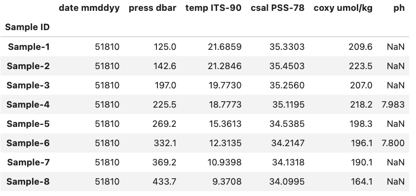
As an example lets say that we wanted to compare each sample in df with the equivalent sample in df2 (based on their row index value) and find those where the df sample’s oxygen concentration coxy umol/kg is less than df2. To do this we start by comparing the two DataFrame.
df.loc[:, "coxy umol/kg"] < df2.loc[:, "coxy umol/kg"]
Below you can see the output of the code.
Sample ID
Sample-1    False
Sample-2     True
Sample-3     True
Sample-4     True
Sample-5    False
Sample-6     True
Sample-7     True
Sample-8     True
Name: coxy umol/kg, dtype: bool
So we can see that there are two samples, Sample-1 and Sample-5, where the oxygen concentration is smaller for df compared to df2. If we inspect both DataFrames we can easily see that this is the case for Sample-5. However, in the case for Sample-1 it is less clear since we don’t have a comparison between two numeric values and instead NaN < 216.6. When it comes to comparisons between NaN values and numeric values by default it will always return False. If we were to instead check for samples where df has a greater oxygen concentration we would run into the same result for Sample-1 i.e. the result would be False
df.loc[:, "coxy umol/kg"] > df2.loc[:, "coxy umol/kg"]
Sample ID
Sample-1    False
Sample-2    False
Sample-3    False
Sample-4    False
Sample-5     True
Sample-6    False
Sample-7    False
Sample-8    False
Name: coxy umol/kg, dtype: bool
Column Specification
If you do not specify a column to compare and instead do e.g.
df.loc[:] < df2.loc[:]you will get a comparison of every column and aDataFramecontaining those values as an output:df.loc[:] < df2.loc[:]date mmddyy press dbar temp ITS-90 csal PSS-78 coxy umol/kg ph Sample ID Sample-1 True False True True False False Sample-2 True False True True True False Sample-3 True False True True True False Sample-4 True False True True True True Sample-5 True False True True False False Sample-6 True False True True True False Sample-7 True False True True True False Sample-8 True False True True True False
Sorting
There may also come a time when we want to see the data sorted by some criterion in order to explore potential patterns and order statistics of the entries based on a relation. For example, we might want to order a DataFrame by the depth that a sample was recovered from. Note: we can also sort the order of the columns based on their names
There are two primary methods to sort a DataFrame either by the index or by a value. The index is rather straight forward, you use the method sort_index() to sort the DataFrame and provide an axis (0=row, 1=columns). We can reuse df and since the index is already sorted we can sort the order of the columns instead.
df.sort_index(axis=1)
With the output:
           coxy umol/kg  csal PSS-78  date mmddyy     ph  press dbar  temp ITS-90
Sample ID
Sample-1            NaN      35.0636        40610  7.951       239.8      18.9625
Sample-2          192.3      34.6103        40610    NaN       280.7      16.1095
Sample-3          190.8      34.2475        40610    NaN       320.1      12.9729
Sample-4          191.3      34.1884        40610  7.780       341.3      11.9665
Sample-5          203.5      34.1709        40610    NaN       360.1      11.3636
Sample-6          193.7      34.1083        40610    NaN       385.0      10.4636
Sample-7          156.5      34.0567        40610    NaN       443.7       8.5897
Sample-8          110.7      34.0424        40610  7.496       497.8       7.1464
Here we can see that we’ve ordered the columns alphabetically.
If we want to instead order the DataFrame based on the value in a particular column or row we instead use sort_values(). We can again use the pressure i.e. ‘press dbar’ column as an example and sort the rows by greatest to smallest pressure value.
df.sort_values(by='press dbar', axis=0, ascending=False)
Will produce the reorder DataFrame as the output:
           date mmddyy  press dbar  temp ITS-90  csal PSS-78  coxy umol/kg     ph
Sample ID
Sample-8         40610       497.8       7.1464      34.0424         110.7  7.496
Sample-7         40610       443.7       8.5897      34.0567         156.5    NaN
Sample-6         40610       385.0      10.4636      34.1083         193.7    NaN
Sample-5         40610       360.1      11.3636      34.1709         203.5    NaN
Sample-4         40610       341.3      11.9665      34.1884         191.3  7.780
Sample-3         40610       320.1      12.9729      34.2475         190.8    NaN
Sample-2         40610       280.7      16.1095      34.6103         192.3    NaN
Sample-1         40610       239.8      18.9625      35.0636           NaN  7.951
Key Points
Select columns by using
["column name"]or rows by using thelocattributeSort based on values in a column by using the
sort_valuesmethod
DataFrame Analysis
Overview
Teaching: 20 min
Exercises: 0 minQuestions
What are some common attributes for Pandas
DataFrames?What are some common methods for Pandas
DataFrames?How can you do arithmetic between two Pandas columns?
Objectives
Learn how to access
DataFrameattributesLearn how to get statistics on a loaded
DataFrameLearn how to sum two Pandas
DataFramecolumns together
DataFrame Attributes & Arithmetic
Once you have loaded in one or more DataFrames you may want to investigate various aspects of the data. This could be by looking at the shape of the DataFrame or the mean of a single column. This could also be through arithmetic between different DataFrame columns (i.e. Series). The following episode will focus on these two concepts and will help you better understand how you can analyze the data you have loaded into Pandas.
DataFrame Attributes
It is often useful to quickly explore some of the descriptive attributes and statistics of the dataset that you are working with. For instance, the shape and datatypes of the DataFrame, and the range, mean, standard deviation, etc. of the rows or columns. You may find interesting patterns or possibly catch errors in your dataset this way. As we will see, accessing these attributes and computing the descriptive statistics is easy with pandas.
DataFrames have a number of attributes associated with them. With respect to exploring your dataset, perhaps the 4 most useful attributes are summarized in the table below:
| Attribute | Description |
|---|---|
shape |
Returns a tuple representing the dimensionality of the DataFrame. |
size |
Returns an int representing the number of elements in this object. |
dtypes |
Returns the data types in the DataFrame. |
columns |
Returns a Series of the header names from the DataFrame |
A list of all the DataFrame attributes can be found on the pandas website (Link to DataFrame Docs).
Inspecting Data Types
DataFrame types are important since they will determine what methods can be used. For example you can’t compute the mean of a Object column that contains strings (i.e. words).
One attribute that we have already used previously was the columns attribute that returns the name of each column header
df.columns
That returns:
Index(['Sample ID', 'date mmddyy', 'press dbar', 'temp ITS-90', 'csal PSS-78',
       'coxy umol/kg', 'ph'],
      dtype='object')
However, what if we wanted to see the data type associated with each column header? Luckily, there is a quick and easy way to do this by accessing the dtypes attribute. dtypes is a series maintained by each DataFrame that contains the data type for each column inside a DataFrame. As an example if we want to access the dtypes attribute the DataFrame called df (seen below) we can access the dtypes of the DataFrame.
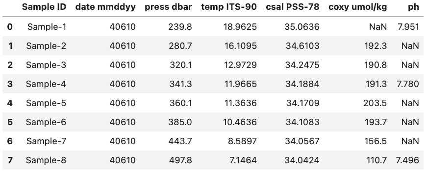
df.dtypes
This will produce the output:
Sample ID        object
date mmddyy       int64
press dbar      float64
temp ITS-90     float64
csal PSS-78     float64
coxy umol/kg    float64
ph              float64
dtype: object
Data Types
Remember that Pandas has a number of different data types:
Python Type Equivalent Pandas Type Description string or mixedobjectColumns contain partially or completely made up from strings intint64Columns with numeric (integer) values. The 64 here refers
to size of the memory space allocated to this typefloatfloat64Columns with floating points numbers (numbers with decimal points) boolboolTrue/False values datetimedatetimeDate and/or time values
While Pandas is usually pretty good at getting the type of a column right sometimes you might need help it by providing the type when the data is loaded in or by converting it to a more suitable format.
As an example we are going to use the column ‘date mmddyy’ to create a new column just called ‘date’ that has the type datetime.
To start we can convert the information stored in ‘date mmddyy’ into a new Series with the datetime type. To do this we call the to_datetime method and provide the Series we want it to convert from as a parameter. Additionally we also need to specify the format that our date format is in. In our case we have month day and then year with each denoted by two numbers and no separators. To tell to_datetime that our data is formatted in this way we pass ‘%m%d%y’ to the format parameter. This format parameter input is based on native python string conversion to datetime format more information can be found on on the python docs (Link to string to datetime conversion docs)
More information on the to_datetime method can be found on the Pandas website (Link to to_datetime method docs).
pd.to_datetime(df['date mmddyy'], format='%m%d%y')
0   2010-04-06
1   2010-04-06
2   2010-04-06
3   2010-04-06
4   2010-04-06
5   2010-04-06
6   2010-04-06
7   2010-04-06
Name: date mmddyy, dtype: datetime64[ns]
Now that we have the correct output format we can create a new column to hold the converted data in by creating a new named column. We will also drop the previously used ‘date mmddyy’ column to prevent confusion. Lastly, we will display the types for each of the columns to check that everything went the way we wanted it to.
df["date"] = pd.to_datetime(df['date mmddyy'], format='%m%d%y')
df = df.drop(columns=["date mmddyy"])
df.dtypes
Sample ID               object
press dbar             float64
temp ITS-90            float64
csal PSS-78            float64
coxy umol/kg           float64
ph                     float64
date            datetime64[ns]
dtype: object
For reference this is what the final DataFrame looks like. Note that the date column is at the right side of the DataFrame since it was added last.
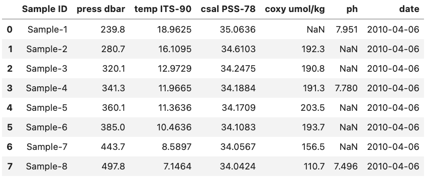
DataFrame Methods
When dealing with a DataFrame there are a variety of built-in methods to help summarize the data found inside it. These are accessible using e.g. df.method() where df is a DataFrame. A list of some of these methods can be seen below:
| Method | Description |
|---|---|
head() |
Return the first n rows. |
tail() |
Return the last n rows. |
min(), max() |
Computes the numeric (for numeric value) or alphanumeric (for object values) row-wise min, max in a Series or DataFrame. |
sum(), mean(), std(), var() |
Computes the row-wise sum, mean, standard deviation and variance in a Series or DataFrame. |
nlargest() |
\tReturn the first n rows of the Series or DataFrame, ordered by the specified columns in descending order. |
count() |
Returns the number of non-NaN values in the in a Series or DataFrame. |
value_counts() |
Returns the frequency for each value in the Series. |
describe() |
Computes row-wise statistics. |
A full list of methods for DataFrames can be found in the Pandas docs (Link to DataFrame Docs).
Some of these we have already dealt with e.g. value_counts() while others are fairly self descriptive e.g. head() and tail(). Below we will deal with one method mean() that is a good representative for how most of the methods work and another describe() that is a bit more tricky.
mean() Method
The mean() method calculates the mean for an axis (rows = 0, columns = 1). As an example let’s return to our previous DataFrame df.
If we want to find the mean of all of our numeric columns we would give the following command
df.mean(numeric_only=True)
This will produce the output:
press dbar      358.562500
temp ITS-90      12.196838
csal PSS-78      34.311013
coxy umol/kg    176.971429
ph                7.742333
dtype: float64
Note: only the columns with numeric data types had their means calculated.
Single Column (
Series) MethodsIf we only want the mean of a single column we would instead give the
mean()method a single column (i.e. aSeries). This could be done for the latitude column in the example above via the code bitdf['Latitude'].mean()which would return a single value 31.09682 which is the mean of that column (as seen above).
Other methods like max(), var(), and count() function in much the same way.
describe() Method
A method that is a bit more tricky to understand is the describe() method. This method provides a range of statistics about the DataFrame depending on the contents. For example if we were to run describe() on the previously mentioned DataFrame called df using the code bit below.
Single Column (
Series) MethodsBy default the
describe()method will only use numeric columns. To tell it to use all columns regardless of whether they are numeric or not we have to setinclude='all'-
df.describe(include='all', datetime_is_numeric=True)
We would get the output:
       Sample ID  press dbar  temp ITS-90  csal PSS-78  coxy umol/kg  \
count          8    8.000000     8.000000     8.000000      7.000000
unique         8         NaN          NaN          NaN           NaN
top     Sample-1         NaN          NaN          NaN           NaN
freq           1         NaN          NaN          NaN           NaN
mean         NaN  358.562500    12.196838    34.311013    176.971429
min          NaN  239.800000     7.146400    34.042400    110.700000
25%          NaN  310.250000     9.995125    34.095400    173.650000
50%          NaN  350.700000    11.665050    34.179650    191.300000
75%          NaN  399.675000    13.757050    34.338200    193.000000
max          NaN  497.800000    18.962500    35.063600    203.500000
std          NaN   83.905762     3.853666     0.353064     32.726376

              ph                 date
count   3.000000                    8
unique       NaN                  NaN
top          NaN                  NaN
freq         NaN                  NaN
mean    7.742333  2010-04-06 00:00:00
min     7.496000  2010-04-06 00:00:00
25%     7.638000  2010-04-06 00:00:00
50%     7.780000  2010-04-06 00:00:00
75%     7.865500  2010-04-06 00:00:00
max     7.951000  2010-04-06 00:00:00
std     0.229827                  NaN
Here we get statistics regarding e.g. the mean of each column, how many non-NaN values are found in the columns, the standard deviation of the column, etc. The percent values correspond to the different percentiles of each column e.g. the 25% percentile. The NaN values are since we can’t get e.g. the mean() of an object type column. More information about the describe() method can be found on the Pandas website (Link to describe() method docs).
DataFrame Arithmetic
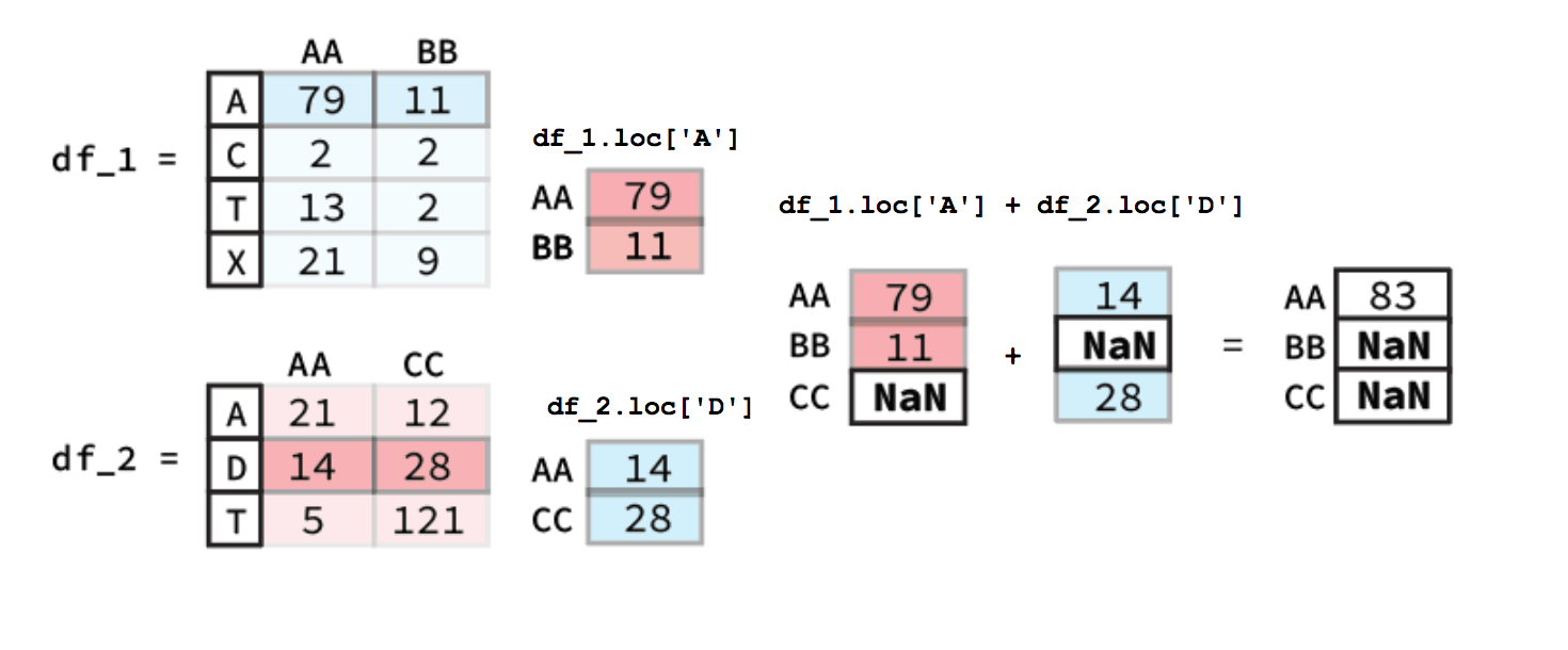
There may also come a time where we might want to do arithmetic between two different DataFrame columns or rows. Luckily, Pandas helps make this very simple. For example if had two DataFrames like the ones below and we wanted to add the ‘AA’ columns together we would simply use the following code bit:
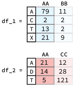
df_1["AA"] + df_2["AA"]
To calculate this Pandas will first align the two columns (Series) based on their indexes. Following this any indexes that contain values in both Series will have their sum calculated. However, for indexes where one of the Series value is NaN the output value will be NaN. A diagram of this process is shown below:
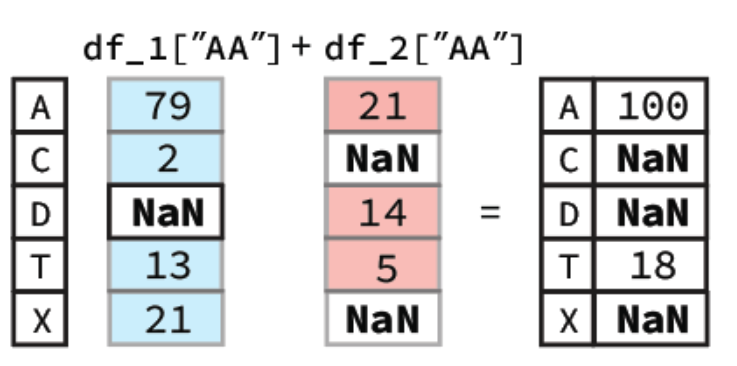
In our notebook we would get a Series as our output:
A    100.0
C      NaN
D      NaN
T     18.0
X      NaN
Name: AA, dtype: float64
DataFrameRow ArithmeticCalculating the sum of different rows is pretty similar to column-wise calculations. The key difference is that you must used a method of selecting rows e.g.
.locan example figure is shown below.
Beyond just individual columns or rows you can also apply the same method to do arithmetic between two entire DataFrames. The only thing that changes is that both the column and the index must be found in a in order for there to be an output. You can imagine that doing arithmetic between two entire DataFrame’s functions in much the same way if you did it column by column and then turned all the resulting column Series into a new DataFrame.
Broadcasting
Pandas also allows you to do arithmetic operations between a DataFrame or Series and a scalar (i.e. a single number). If you were to do the following code bit using the ‘AA’ column from the previously described DataFrame called df_1
df_1["AA"] + 0.3
You would get the output:
A    79.3
C     2.3
T    13.3
X    21.3
Name: AA, dtype: float64
Here you essentially just add 0.3 to each entry in the Series. The same occurs if you were to do it for a whole DataFrame with 0.3 being added to each entry. Note: this only works for DataFrames that are entirely numeric, if there are any object columns you will get an error message.
Key Points
Using
.dtypesto get the types of each column in aDataFrameTo get general statistics on the DataFrame you can use the
describemethodYou can add a constant to a numeric column by using the
column + constant
Real Example Cleaning
Overview
Teaching: 10 min
Exercises: 10 minQuestions
How do you clean an example dataset?
How do you deal with missing data?
How do you fix column type mismatches?
Objectives
Clean an example dataset using both previously described concepts and some new ones
Cleaning Real Data
The previous episodes have focused on key concepts with small datasets and/or made up data. However, these examples can only take you so far. For this reason the remaining lessons and examples will be focused on an actual dataset from the Hawaiian Ocean Time-Series (HOT) data website (Link to HOT Data Website). This website allows you to query data generated by the time-series through various modules.
The Hawaiian Ocean Time-Series has been collecting samples from station ALOHA located just North of Oahu since 1988. The map below shows the exact location where the samples we will be using originate from.

(Original image from: https://www.soest.hawaii.edu/HOT_WOCE/bath_HOT_Hawaii.html)
Going forward we are going to be using data from HOT between the 1st of January 2010 to the 1st of January 2020. This particular data we are going to be utilizing comes from bottle extractions between depths 0 to 500m. The environmental variables that we will be looking at include:
| Column name | Environmental Variable |
|---|---|
| botid # | Bottle ID |
| date mmddyy | Date |
| press dbar | Pressure |
| temp ITS-90 | Temperature |
| csal PSS-78 | Salinity |
| coxy umol/kg | Oxygen concentration |
| ph | pH |
| phos umol/kg | Phosphate concentration |
| nit umol/kg | Nitrate + Nitrite concentration |
| no2 nmol/kg | Nitrite concentration |
| doc umol/kg | Dissolved Organic Carbon concentration |
| hbact #*1e5/ml | Heterotrophic Bacteria concentration |
| pbact #*1e5/ml | Prochlorococcus numbers |
| sbact #*1e5/ml | Synechococcus numbers |
The data contains over 20000 individual samples. To analyze the data we are going to clean it up. Then, in the next episode we will analyze and visualize it. To do this we will be using some of tricks we have already learn while also introducing some new things. Note: The dataset we are using has been modified from its original format to reduce the amount of cleaning up we need to do.
Cleaning Up
DataFrame Content Cleanup
During our initial clean up we will only load in the first few rows of our dataset entire DataFrame. This will make it easier to work with and less daunting.
pd.read_csv("./data/hot_dogs_data.csv", nrows=5)
This will show us the DataFrame seen below:

From this we can see a few things:
- There are a lot of -9 values
- This is likely to denote Null values in the dataset
- The last column (to the right of the no2 column) doesn’t seem to contain a header or any data
Both of these issues can easily be fixed using Pandas and things we’ve learn previously.
To start off lets fix the first problem we saw which was was the large number of -9 values in the dataset. These are especially strange for some of the columns e.g. how can there be a negative concentration of hbact i.e. heterotrophic bacteria? This is a stand in for places where no measurement was obtained.
Treating -9 values as NaN values when loading data
To start off try fixing the read_csv() method so that all -9 values are treated as NaN values. If you are stuck try going back to the episode on this topic (Link to loading data episode).
Solution
To fix this we can add the parameter
na_values=-9to theread_csv()method giving us the following code bit.pd.read_csv("./data/hot_dogs_data.csv", nrows=5, na_values=-9)Below shows how our
DataFramenow looks:
With this we have fixed the problematic -9 values from our initial DataFrame.
Temperature Column
The temperature column could technically contain -9 values. However, all temperature measurements were above 0 so this is not an issue.
The second problem we identified was that there was an extra column (with no header) made up of only NaN values. This is probably an issue with the original file and if we were to take a look at the raw .csv file we find that each row ends with a ‘,’. This causes read_csv to assume that there is another column with no data since it looks for a new line character (\n) to denote when to start a new row.
There are various methods to deal with this. However, we are going to use a relative simple method that we’ve already learn. As we discussed in a previous episode pandas DataFrames have a method to drop columns (or indexes) called drop. Where if we provide it with the correct inputs it can drop a column based on its name. Knowing this we can chain our read_csv method with the drop method so that we load in the blank column and then immediately remove it.
Dropping the blank column
The final command we will be using can be seen below. However, the columns parameter is missing any entries in its list of columns to drop. You will be fixing this by adding the name of the column that is empty (hint: the name isn’t actually empty).
pd.read_csv("./data/hot_dogs_data.csv", nrows=5, na_values=-9).drop(columns=[])To get the name of the column we will want to utilize a
DataFrameattribute that we have already discussed that provides us with the list of names in the same order they occur in theDataFrame. If you are stuck check the previous episode where we discussed this (Link to previous episode).Solution
To get the name of the columns we can simply access the
columnsSeriesattribute that everDataFramehas. This can be done either through chaining it after ourread_csvmethod or by store it in a variable and then call the method using that variable. Below we use the chain approach.pd.read_csv("./data/hot_dogs_data.csv", nrows=5, na_values=-9).columnsIndex(['botid #', ' date mmddyy', ' press dbar', ' temp ITS-90', ' csal PSS-78', ' coxy umol/kg', ' ph', ' phos umol/kg', ' nit umol/kg', ' doc umol/kg', ' hbact #*1e5/ml', ' pbact #*1e5/ml', ' sbact #*1e5/ml', ' no2 nmol/kg', ' '], dtype='object')The last entry in the
Seriesis our ‘blank’ column i.e.' '. We add this as the only entry to our drop method and get the following code bit.pd.read_csv("./data/hot_dogs_data.csv", nrows=5, na_values=-9).drop(columns=[" "], axis=1)This then gives us the output
DataFrameseen below:
With this we have fixed some of the initial issues related to our dataset. It should be noted that there might still exist other issues with our dataset since we have only relied on the first few rows.
Column Names
Checking the
columnsattribute even if nothing immediately looks wrong can be good in order to spot e.g. blank spaces around column names that can lead to issues.
One final thing that we are going to do that is not quite “clean up” but nonetheless important is to set our index column when we load the data. The column we are going to use for this is the ‘botid #’ column. We can also remove the nrows=5 parameter since we want to load the whole DataFrame starting in the next section.
Setting the index column when loading data
To set the index column we can use a parameter in
read_csvthat was mentioned in a previous episode. See if you can remember it! If you run into trouble you can take a look at the previous episode where it was mentioned (Link to prev episode).Solution
To set the index column when we load the data we just have to add the parameter
index_coland set it to ‘botid #’. Note: we have removed thenrows=5parameter in the code bit below since we no longer need it.pd.read_csv("./data/hot_dogs_data.csv", na_values=-9, index_col="botid #").drop(columns=[" "], axis=1)
This gives us a somewhat cleaned up DataFrame that looks like the image below:
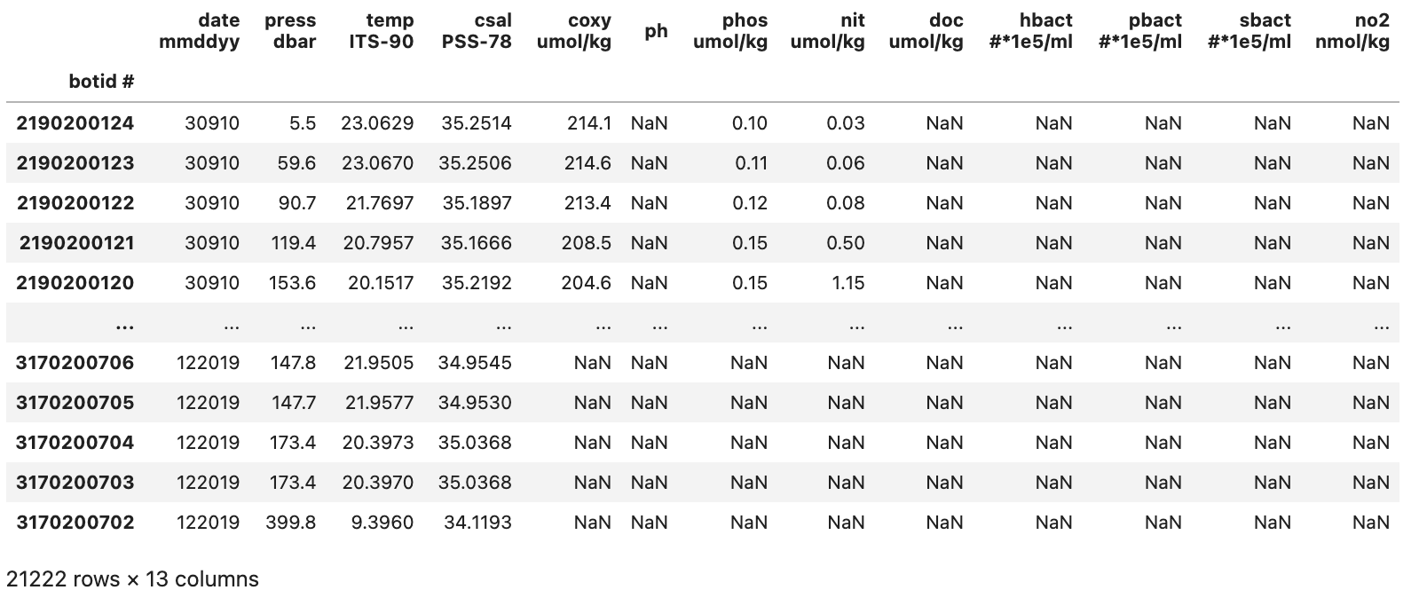
With our initial cleanup done we can now save the current version of our DataFrame to the df variable. This df variable will be used for the next two sections.
DataFrame Column Types
Now that we have fixed the initial issues we could glean from an initial look at the data we can take a look at the types that Pandas assumed for each of our columns. To do this we can access the .dtypes attribute.
df.dtypes
 date mmddyy         int64
 time hhmmss         int64
 press dbar        float64
 temp ITS-90       float64
 csal PSS-78       float64
 coxy umol/kg      float64
 ph                float64
 phos umol/kg      float64
 nit umol/kg       float64
 doc umol/kg       float64
 hbact #*1e5/ml    float64
 pbact #*1e5/ml    float64
 sbact #*1e5/ml    float64
 no2 nmol/kg       float64
dtype: object
Most of the columns have the correct type with the exception of the ‘date mmddyy’ column that has the int64 type. Pandas has a built in type to format date and time columns and conversion of the date column to this datetime type will help us later on.
To change the type of a column from an int64 to a datetime type is a bit more difficult than e.g. a int64 to float64 conversion. This is because we both need to tell Pandas the type that we want it to convert the column’s data to and the format that it is in. For our data this is MMDDYY which we can give to Pandas using format='%m%d%y'. This format parameter can be very complicated but is based on native python more information can be found on the to_datetime method docs (Link to datetime method docs).
The code bit below creates a new column called ‘date’ that contains the same data for each row as is found in the ‘date mmddyy’ column but instead with the datetime64 type. It will not delete the original ‘date mmddyy’ column.
df["collection_date"] = pd.to_datetime(df['date mmddyy'], format='%m%d%y')
df.dtypes
date mmddyy                int64
time hhmmss                int64
press dbar               float64
temp ITS-90              float64
csal PSS-78              float64
coxy umol/kg             float64
ph                       float64
phos umol/kg             float64
nit umol/kg              float64
doc umol/kg              float64
hbact #*1e5/ml           float64
pbact #*1e5/ml           float64
sbact #*1e5/ml           float64
no2 nmol/kg              float64
date              datetime64[ns]
dtype: object
We can see from the output that we have all of our previous columns with the addition of a ‘date’ column with the type datetime64. If we take a look at the new column we can see that it has a different formatting compared to the ‘date mmddyy’ column
df["collection_date"]
botid #
2190200124   2010-03-09
2190200123   2010-03-09
2190200122   2010-03-09
2190200121   2010-03-09
2190200120   2010-03-09
                ...
3170200706   2019-12-20
3170200705   2019-12-20
3170200704   2019-12-20
3170200703   2019-12-20
3170200702   2019-12-20
Name: collection_date, Length: 21222, dtype: datetime64[ns]
Now that we’ve added this column (which contains the same data as found in ‘date mmddyy’ just in a different format) there is no need for the original date mmddyy column so we can drop it.
df = df.drop(columns=["date mmddyy"])
DataFrame Overview
A final thing we will want to do before moving on to the analysis episode is to get an overview of our DataFrame as a final way of checking to see if anything is wrong. To do this we can use the describe() method which we discussed earlier.
df.describe()
         time hhmmss    press dbar   temp ITS-90   csal PSS-78  coxy umol/kg  \
count   21222.000000  21222.000000  21222.000000  21210.000000   3727.000000
mean   103238.977523    119.381105     21.570407     35.020524    198.222297
std     68253.013809    120.193833      4.961006      0.382516     27.787824
min         3.000000      0.800000      6.055800     34.018800     30.900000
25%     40625.000000     25.500000     20.625800     34.922500    199.350000
50%    101309.000000     89.700000     23.109450     35.138700    207.200000
75%    154822.000000    150.900000     24.742175     35.281500    212.000000
max    235954.000000    500.000000     28.240100     35.556400    230.900000

               ph  phos umol/kg  nit umol/kg  doc umol/kg  hbact #*1e5/ml  \
count  885.000000   2259.000000  2253.000000   868.000000      750.000000
mean     7.956939      0.448331     5.505113    63.688341        3.933479
std      0.158210      0.638772     9.159562    10.287748        1.173908
min      7.366000      0.000000     0.000000    41.270000        1.481000
25%      7.898000      0.070000     0.020000    55.467500        2.976250
50%      8.035000      0.120000     0.240000    67.395000        4.042000
75%      8.065000      0.520000     6.620000    72.282500        4.809500
max      8.105000      2.610000    35.490000    80.460000        7.889000

       pbact #*1e5/ml  sbact #*1e5/ml  no2 nmol/kg
count      749.000000      750.000000          0.0
mean         1.364606        0.010932          NaN
std          0.938620        0.011851          NaN
min          0.000000        0.000000          NaN
25%          0.337000        0.000000          NaN
50%          1.643000        0.009000          NaN
75%          2.176000        0.016000          NaN
max          3.555000        0.091000          NaN
A look at the output shows us that the ‘no2 nmol/kg’ column does not contain any useable data based on its count value being 0. This then leads to the NaN for e.g. the min and max values. Since this column doesn’t contain any information of interest we can drop it to clean up our DataFrame.
df = df.drop(columns=["no2 nmol/kg"])
With this done our data is reasonably cleaned up and we have the DataFrame seen in the image below:
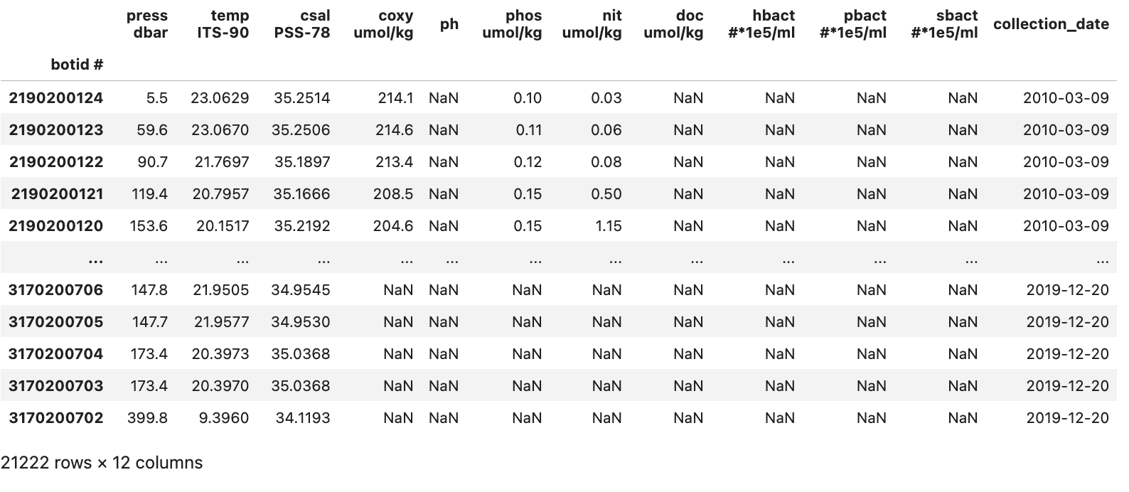
We can now move on to the analysis and visualization of the data in our DataFrame.
Summary
With this we’ve clean up our initial dataset. To summarize we have:
- Replaced the -9 placeholder for Null values with NaN values
- Fixed an issue with an extra column containing no data
- Added a custom row index
- Converted the data in ‘date mmddyy’ to a Pandas supported datetime type
- Dropped two columns:
- ‘date mmddyy’ column since the new ‘date’ column contains the same data but in a better type
- ‘no2 nmol/kg’ column since it contained no data
Key Points
Cleaning a dataset is an iterative process that can require multiple passes
Keep in mind to restart the kernel when cleaning a dataset to make sure that your code encompasses all the cleaning needed.
Real Example Analysis
Overview
Teaching: 10 min
Exercises: 10 minQuestions
How do you visualize data from a
DataFrame?How do you group data by year and month?
How do you plot multiple measurements in a single plot?
Objectives
Learn how to plot the cleaned data
Learn how to subset and plot the data
Learn how to using the groupby method to visualize yearly and monthly changes
Analyzing Real Data
This episode continues from the previous one and utilizes the final DataFrame described there.
Analysis
Before we get started on our analysis let us take stock of how much data we have for the various columns. To do this we can use two DataFrame methods that we’ve previously used.
First we can check how many rows of data we have in total. We can check this easily through the shape attribute of the DataFrame
df.shape
(21222, 13)
From this we can see that we have 21222 rows in our data and 13 columns. So at most we can have 21222 rows of data for each column. However, as we saw during the cleaning phase there are NaN values in our dataset so many of our columns won’t contain data in every row.
To check how many rows of data we have for each column we can again use the describe() method. It will count how many row of data are not NaN for each column. To reduce the size of the output we will use loc to only view the counts for each column.
df.describe().loc["count",:]
time hhmmss       21222.0
press dbar        21222.0
temp ITS-90       21222.0
csal PSS-78       21210.0
coxy umol/kg       3727.0
ph                  885.0
phos umol/kg       2259.0
nit umol/kg        2253.0
doc umol/kg         868.0
hbact #*1e5/ml      750.0
pbact #*1e5/ml      749.0
sbact #*1e5/ml      750.0
Name: count, dtype: float64
As we can see we have highly variable amounts of data for each of our column. We will ignore pressure since it is roughly a depth estimate. These fit fairly neatly into three groups:
- Data that is found in almost all rows
- Temperature
- Salinity
- Data that is found in around 2000-4000 samples
- Oxygen
- Phosphorus
- Nitrate+Nitrite
- Data that is found in fewer than 1000 samples
- pH
- Dissolved organic carbon
- Heterotrophic bacteria
- Prochlorococcus
- Synechococcus
Note here that pressure is roughly akin to “depth” so we won’t be using it.
GroupBy and Visualization
To start off we can focus on the measurements that we have plenty of data for.
Plotting Temperature
We can quickly get a matplotlib visualization for temperature by calling the
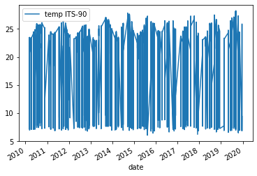
plotmethod from ourDataFrame. We can tell it what columns we want to use as the x axis and y axis via the parametersxandy. Thekindparameter lets theplot()method know what kind of plot we want e.g. line or scatter. For more information about the plot function check out the docs (Link to plot method docs).df.plot(x="date", y="temp ITS-90", kind="line")Solution
Below is the output plot
However, the plot we get is very messy. We see a lot of variation from around 25°C to 7°C year to year and the lines are clustered very tightly together.
Plotting Surface Temperature
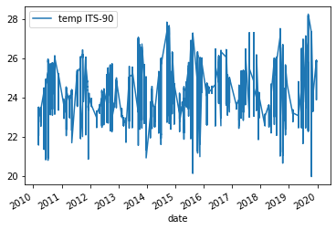
Part of the reason we got this messy plot is because we are utilizing all the temperature values in our dataset, regardless of depth (i.e. pressure). To resolve some of the variation we can ask Pandas to only plot data that is from roughly the top 100m of the water column this would be roughly any rows that come from pressures of less than 100 dbar.
surface_samples = df[df["press dbar"] < 100]
surface_samples.plot(x="date", y="temp ITS-90", kind="line")
Solution
Below is the output plot
Now we can see that we have removed some of the variation we saw in the previous figure. However, it is still somewhat difficult to make out any trends in the data. One way of dealing with this would be to e.g. get the average temperature for each year and then plot those results.
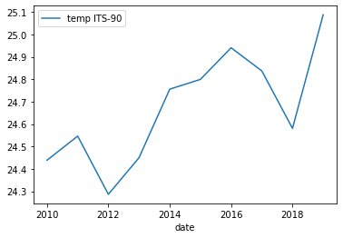
To this we will introduce a new method called groupby which allows us to run calculations like mean() on groups we specify. For us we want to get the mean temperature for each year. Thanks to our previous work in setting up the date column type this is very easy. We can also reuse surface_samples to only get samples from the upper 100m of the water column.
grouped_surface_samples = surface_samples.groupby(df.date.dt.year).mean()
        time hhmmss  press dbar  temp ITS-90  csal PSS-78  coxy umol/kg  \
date
2010  111193.170920   37.517015    24.438342    35.282562    213.306024
2011  108457.713156   40.025449    24.545986    35.225530    210.137566
2012  103491.885435   37.503730    24.286195    35.200273    211.909375
2013  110479.360743   38.544562    24.449899    35.302473    211.057143
2014  107638.631016   40.763369    24.755485    35.287073    211.538974
2015  108635.305970   37.930929    24.799153    35.210472    210.160287
2016  101880.099391   37.814300    24.940249    34.995771    208.771186
2017  106559.737030   36.499374    24.836940    35.000984    211.143750
2018  103767.267879   37.064727    24.580730    34.999648    213.029371
2019  104902.595131   38.461587    25.087561    34.805649    212.239130

            ph  phos umol/kg  nit umol/kg  doc umol/kg  hbact #*1e5/ml  \
date
2010  8.063846      0.075842     0.033465    73.810154        4.614946
2011  8.072089      0.056455     0.029464    74.384000        4.651204
2012  8.061535      0.114953     0.018224    72.578871        4.787081
2013  8.064927      0.087264     0.026981    71.548413        4.778000
2014  8.069786      0.065983     0.025652    72.237091        4.845439
2015  8.065829      0.071795     0.029211    70.894154        4.838659
2016  8.072237      0.068108     0.055676    72.562131        4.467324
2017  8.064918      0.052946     0.033514    70.556863        4.744976
2018  8.054656      0.060000     0.085250          NaN        4.555553
2019  8.061786      0.060093     0.021667          NaN        5.084833

      pbact #*1e5/ml  sbact #*1e5/ml
date
2010        1.909351        0.014351
2011        1.783857        0.019388
2012        1.968270        0.015351
2013        2.345216        0.020162
2014        2.223146        0.018927
2015        2.182341        0.018386
2016        2.127529        0.014471
2017        2.109878        0.019927
2018        2.035622        0.020711
2019        2.123119        0.015214
We see now that the new DataFrame generated by groupby() and mean() contains the mean for each year for each of our columns.
Plotting Yearly Surface Temperature
Now we can just run the same plot method as previously but using
grouped_surface_samplesinstead ofsurface_samples.grouped_surface_samples.plot(x="date", y="temp ITS-90", kind="line")Solution
Below is the output plot
Now it looks a lot smoother, but now we have another issue. We’ve smoothed out any month to month variations that are present in the data. To fix this we can instead use the groupby method to group by year and month.
grouped_surface_samples = surface_samples.groupby([(surface_samples.date.dt.year),(surface_samples.date.dt.month)]).mean()
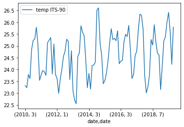
Plotting Monthly Surface Temperature
If we plot this we get a month by month plot of temperature variations.
grouped_surface_samples.plot(y="temp ITS-90", kind="line")Solution
Below is the output plot
While we have been focusing on temperature there is no reason that we can’t redo the same plots that we have been making with measurements other than temperature. We can also plot multiple measurements at the same time if we want to as well.
Plotting Monthly Surface Temperature
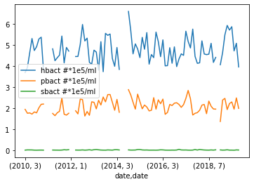
To test this we will try plotting the abundance of Prochlorococcus, Synechococcus, and heterotrophic bacteria.
grouped_surface_samples.plot(y=["hbact #*1e5/ml", "pbact #*1e5/ml",
                                "sbact #*1e5/ml"], kind="line")
Solution
Below is the output plot
With that we plotted looked various methods of plotting the data we have in our dataset. We’ve also learned how to group different measurements depending on when the measurement was taken. If you are interested you can keep testing different methods of grouping the data or plotting some of the measurements that we did not use e.g. pH or dissolved organic carbon (doc umol/kg).
Hopefully throughout this lesson you have learned some useful skills in order to both analyze your data and document your analysis and any code that you used. There is plenty of things that we did not have time to go over so make sure to keep learning!
Key Points
Grouping data by year and months is a powerful way to identify monthly and yearly changes
You can easily add more measurements to a single plot by using a list
There is a lot we didn’t cover here, so take a look at the Matplotlib docs (Link to Matplotlib docs) and other libraries that can allow you to make dynamic plots e.g. Plotly (Link to Plotly docs)
