Loading and Handling Pandas Data
Overview
Teaching: 20 min
Exercises: 0 minQuestions
How are Pandas data structures setup?
How to load data into Pandas?
How to write data from Pandas to a file
Objectives
Understand the usefulness of Pandas when loading data
Understand how to load data and deal with common issues
Pandas Data Structures
For this episode you should follow along inside the Jupyter notebook associated with this episode. The jupyter notebooks for this entire lesson can be found in Binder (Link to lesson’s Binder website). You will have to navigate to the “notebook” directory in the file browser to find the notebook associated with this episode.
Before we start loading data into Pandas we need to become familiar with 2 of the primary data structures of Pandas:
- Series
- DataFrames
The reason we use Series and DataFrames rather than native python data structures to hold our data is because there are additional attributes and methods associated with Series and DataFrames that will be useful for wrangling and analytics. One of the primary benefits of Series and DataFrames over native python data structures is that it is a very natural way to describe a data set in an excel-like manner by referencing the rows and columns of our data with labels of our choosing.
Pandas Series Vs. DataFrames
Pandas has two principal data structures, Series and DataFrames. If you are familiar with Microsoft’s Excel application then you can liken Series to single columns (or rows) in an Excel sheet and DataFrames to entire tables (or spreadsheets).
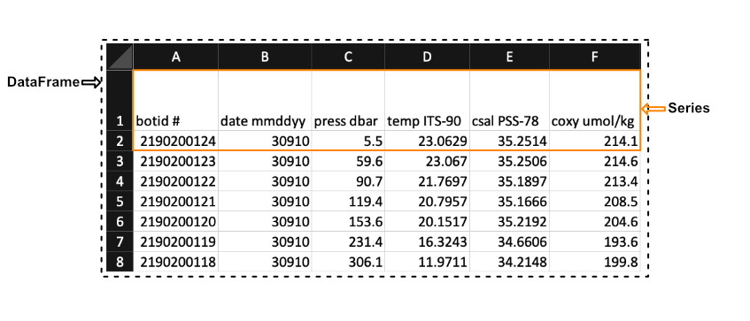
We see in the image above that a Series in the context of Excel could be the first row of the spreadsheet, while a DataFrames would be the entire spreadsheet. In other words, a DataFrames is simply a collection of labeled Series.
Pandas Data Types
When creating a Series Pandas will store all the data as the same type. The mapping from the native python types to what they would be in Pandas is summarized below.
| Python Type | Equivalent Pandas Type | Description |
|---|---|---|
string or mixed |
object |
Columns contain partially or completely made up from strings |
int |
int64 |
Columns with numeric (integer) values. The 64 here refers to size of the memory space allocated to this type |
float |
float64 |
Columns with floating points numbers (numbers with decimal points) |
bool |
bool |
True/False values |
datetime |
datetime |
Date and/or time values |
Pandas DataFrames Basics
DataFrames are essentially ordered collections of Series with two associated Index objects, one to label rows and another to label columns. Reiterating the example mentioned earlier, it helps to think of DataFrames as MS. Excel spreadsheets where each row (or column) as an individual Series.
You can create DataFrames from either loading in a file e.g. a csv file or by converting it from a native Python data structure. However, here we will be focusing on loading data from a file and turning it into a DataFrame.
Creating Pandas
SeriesYou can also create Pandas
Seriesfrom files or native python data structures (Link to more info).
Before we can load in data from a file we need to load the pandas package. Pandas is often imported alongside as pd to reduce the amount of characters needed to use the different methods within it.
import pandas as pd
Loading and Parsing Data
Pandas can load in data from a variety of file formats. However, in most cases you will be loading in data from a plain text file since this is one of the most common and simple ways to store data. Plain text files only contain text without any special formatting or code e.g. .txt, .csv, or .tsv files.
To store data in a plain text file you need a standard way of distinguishing the individual data entries. For example, suppose a file contained the following text:
,column1,column2,column3,
row1,a,b,c
row2,d,e,f
row3,g,h,i
A human would see the text above and may be able to discern the 3 columns and 3 rows and the individual data entries and see that the file contains a table that looks like the one below.
| column 1 | column 2 | column 3 | |
|---|---|---|---|
| row1 | a | b | c |
| row2 | d | e | f |
| row3 | g | h | i |
However, a computer would have no idea how to parse this without any direction; to a computer the text above is just one string of characters. To help the computer parse the text, we could tell it that each data entry is separated by a column and each row is separate by a new line. This way of organizing data is called a plain text file format.
Most of the plain text file formats fall into one of the following two categories: Delimited and Fixed Width
- Delimitted files are organized such that columns and rows are seperated by a certain character called a delimiter
- Fixed width files are those where each entry in a column has a fixed number of characters
We will focus on the delimited .csv file type. csv is an acronym which stands for ‘Comma Separated Values’ and informs us that the column entries are delimited by commas and the rows are delimited by a new line. So, the example we discussed in this cell conforms to the .csv format.
Included in the Pandas toolkit is a collection of parsing functions to read and build DataFrames from data that is stored in a variety of formats. The Pandas function which parses and builds a DataFrame from a generic delimited plain text file is read_csv(). To run read_csv() with the default settings we only need to provide 1 positional argument, the path to the file we want to read. If we wanted to read a file in the same directory as our notebook called p and put the data into a new Pandas DataFrame, df, we would type df = pd.read_csv(p).
However, parsing plain text files can become a complicated procedure. To aid in the process, Pandas provides a lot of optional parameters that may be set when calling the read_csv() function. To learn more, see the read_csv() documentation, which summarizes all of the parameters. We will be covering many of the most important parameters throughout the rest of this lesson.
By default read_csv() will separate data entries when it encounters a comma and will separate rows by new lines encoded by ‘\n’. If we wanted to change this behavior so that read_csv() separates by tabs (encoded with \t), then we can set the optional parameter sep = '\t'. For instance, if we wanted to read the data in the file ‘tsv_example.tsv’, which is a tab separated values file, and save the data in a Pandas DataFrame called df, then we would type:
df = pd.read_csv('data/tsv_example.tsv', sep='\t')
Though read_csv() can handle .tsv files, there is a specific parsing function for .tsv files: read_table(). The difference between read_table() and read_csv() is that the default behavior for the latter is to separate using commas instead of tabs \t. The read_table() documentation is available at this link.
To perform the same operation (that is reading the data in the file tsv_exampletsv and save the data in a Pandas DataFrame called df), we may use the read_table() function without having to define our delimiter, since the default parameters will correctly parse our file.
df = pd.read_table('data/tsv_example.tsv')
Both methods will lead to an equivalent DataFrame.
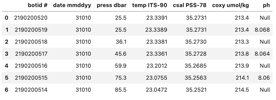
In the previous examples we loaded the entire dataset from the file we gave Pandas. However, when working with large datasets it is good practice to load your data in small pieces before loading the entire dataset to ensure that the file is parsed correctly. Small data sets are more manageable and errors are easier to spot, while large data sets take more time to parse. So, a good workflow is to read a small portion of the data and analyze the resulting data frame to see if you need to modify any of the default behaviors of the read function.
To load only up to a limited number of rows we can use the nrows parameter for both read_table() and read_csv(). For example, the file E3_tara_w1.csv is a csv file with over 200 rows, but if we wanted to read only the first 5 rows of this file we can call the Pandas read_csv() function and set nrows = 5:
df = pd.read_csv('data/tsv_example.tsv', nrows=5)
df.shape # Returns the number of rows and columns of the DataFrame 'df' (rows, columns)
(3, 7)
We see that the DataFrame df, that we saved the data in, has a shape attribute of (3, 7). This means that there are 3 rows (since we set nrows=3) and 7 columns (all the columns of the dataset).
Headers and Indexes
When we loaded the previous datasets read_csv() assumed that the first row in our .csv file contained headers for each of the columns. If we want to load in a dataset that does not contain a header row we can tell read_csv() that there is no header by setting header=None.
df = pd.read_csv("data/noheader_example.csv", header=None)
df
However, this does not mean that the DataFrame does not have headers but rather that Pandas will set them to be an integer value. An example is shown in the figure below:
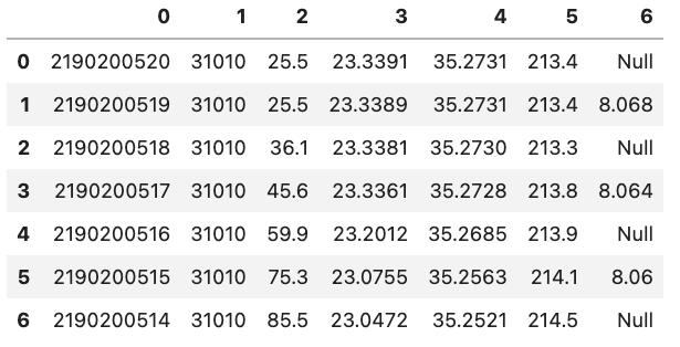
You might also notice that there is also a corresponding integer number in the far left side of each row. This is the index that is essentially the “name” for each row. If we have a column that is specifies each row in the input file we can tell Pandas to use that column instead of the default of using a integer. This can be done by e.g. setting index_col='unique_id' however, if you don’t have any headers you can also specify the column by using its integer location e.g. index_col=0. Note that the integer location of a column goes from left to right and starts at 0.
df = pd.read_csv('data/noheader_example.csv', header=None, index_col=0)
df
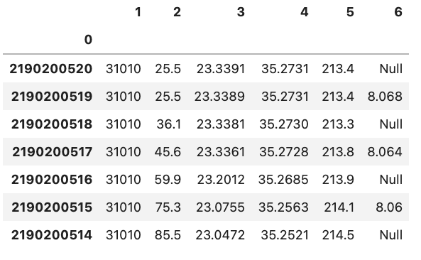
You can change the name of the index column by setting the index name attribute of the dataframe df.index.name = 'unique_id'.
Common Data Loading Problems
Though data storage in plain text files should follow certain formats like .csv for ‘Comma Separated Values’ and .tsv for ‘Tab Separated Values’, there is still some ambiguity on how things like missing entries, and comments should be denoted. For this reason Pandas has implemented functionality into the read_table() and read_csv() to help ‘clean’ plain text data.
Below we will go through two examples of common issues when loading in data.
Missing Values
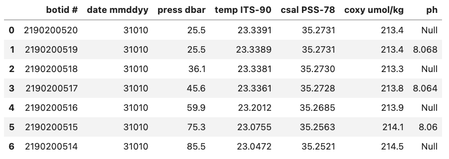
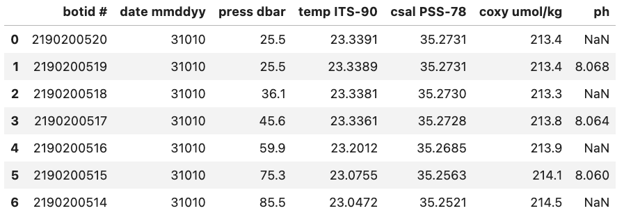
There are often missing values in a real-world data set. These missing entries may be identifiable in the dataset by a number of different tags, like ‘NA’, ‘N.A.’, ‘na’, ‘missing’, etc. It is important to properly identify missing values when creating a DataFrame since certain DataFrame methods rely on the missing values being accounted for. For example, the count() method of a DataFrame returns the number of non missing values in each column. If we want this to be an accurate count, then we need to be sure of pointing out all the tags which represent ‘missing’ to Pandas.
For example, if we were to load in a .csv where missing values are ‘Null’ and not specify this then Pandas will load these values in as objects. To let Pandas know that we want to interpret these values as missing values we can add na_values='Null'.
df = pd.read_csv("data/null_values_example.csv", na_values='Null')
df
Without na_values='Null':
With na_values='Null':
Auto NaN values
Pandas will interpret certain values as being NaN values even without user input. For example if ‘NULL’ is found then Pandas will treat it as a missing value and treat it as a NaN value.
Writing Data in Text Format
Now that we are familiar with the reading mechanisms that Pandas has implemented for us, writing DataFrames to text files follows naturally. Pandas DataFrames have a collection of to_<filetype> methods we can call; we will focus on to_csv(). to_csv() takes the parameter path (the name and location of the file you are writing) and will either create a new file or overwrite the existing file with the same name.
to_csv() has a number of optional parameters that you may find useful, all of which can be found in the Pandas documentation.
df.to_csv('data/new_file.csv')
Key Points
Pandas provides numerous attributes and methods that are useful for wrangling and analyzing data
Pandas contains numerous methods to help load/write data to/from files of different types