What is High Performance Computing (HPC)

Overview

Teaching: 10 min
Exercises: 0 min

Questions

• What is an HPC system?

• What are the components of an HPC system?

Objectives

• Understand the general HPC system architecture

What Is an HPC System?

The words “cloud” and the phrase cluster or high-performance computing (HPC) are used a lot in different contexts and with various related meanings. So what do they mean? And more importantly, how do we use them in our work?

The cloud is a generic term commonly used to refer to computing resources that are a) provisioned to users on demand or as needed and b) represent real or virtual resources that may be located anywhere on Earth. For example, a large company with computing resources in Brazil and Japan may manage those resources as its own internal cloud and that same company may also use commercial cloud resources provided by Amazon or Google. Cloud resources may refer to machines performing relatively simple tasks such as serving websites, providing shared storage, providing web services (such as e-mail or social media platforms), as well as more traditional compute intensive tasks such as running a simulation.

The term HPC system, on the other hand, describes a stand-alone resource for computationally intensive workloads. They are typically comprised of a multitude of integrated processing and storage elements, designed to handle high volumes of data and/or large numbers of floating-point operations (FLOPS) with the highest possible performance. For example, all of the machines on the Top-500 list are HPC systems. To support these constraints, an HPC resource must exist in a specific, fixed location: networking cables can only stretch so far, and electrical and optical signals can travel only so fast.

What else is an HPC system good for

While HPC is typically seen as where you go if you have large problems, HPC clusters can be used for even smaller cases where a single server is all that you need, or you have a reserach problem in which the task is very short, but you need to do tens of thousands of iterations, which is typically known as High Throughput Computing (HTC).

Components of an HPC System

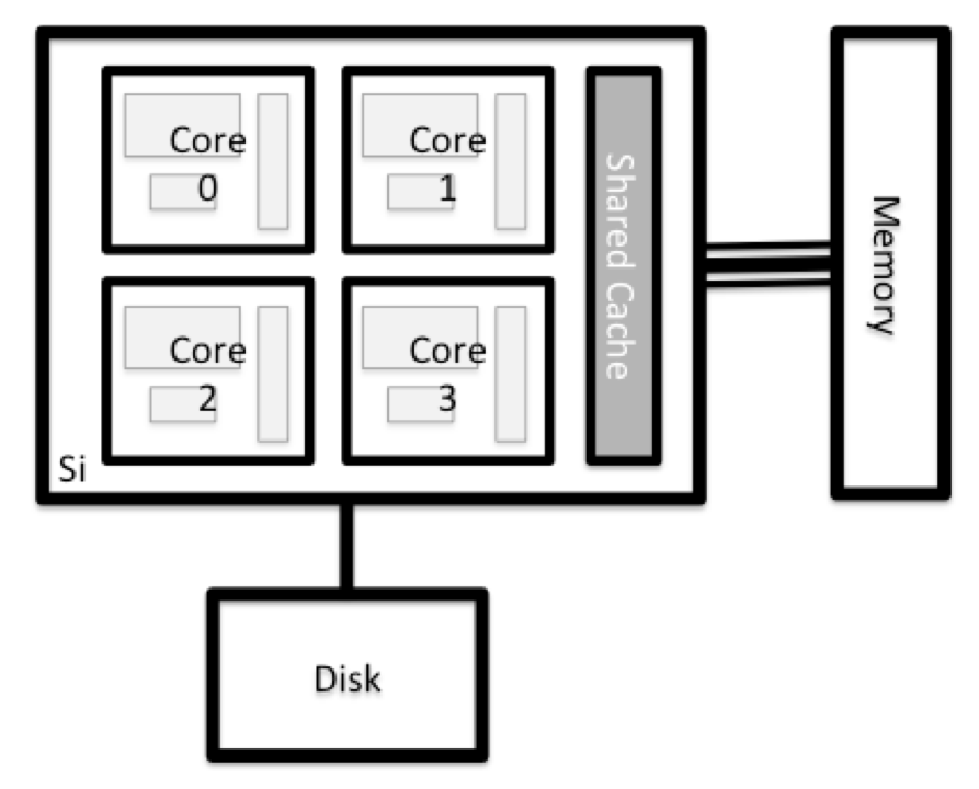
Individual computers that compose a cluster are typically called nodes (although you will also hear people call them servers, computers and machines). On a cluster, there are different types of nodes for different types of tasks.

Anatomy of a Node

All of the nodes in an HPC system have the same components as your own laptop or desktop: CPUs (sometimes also called processors or cores), memory (or RAM), and disk space. CPUs are a computer’s tool for actually running programs and calculations. Information about a current task is stored in the computer’s memory. Disk refers to all storage that can be accessed like a file system. This is generally storage that can hold data permanently, i.e. data is still there even if the computer has been restarted. While this storage can be local (a hard drive installed inside of it), it is more common for nodes to connect to a shared, remote/network fileserver or cluster of servers.

Login Nodes

Serves as an access point to the cluster. As a gateway, it is suitable for uploading and downloading small files.

Data Transfer Nodes

If you want to transfer larger amounts of data to or from a cluster, some systems offer dedicated nodes for data transfers only. The motivation for this lies in the fact that larger data transfers should not obstruct operation of the login node. As a rule of thumb, consider all transfers of a volume larger than 500 MB to 1 GB as large. But these numbers change, e.g., depending on the network connection of yourself and of your cluster or other factors.

Data transfer nodes on Mana

Mana has two such data transfer nodes that are available for use.

Compute Nodes

The real work on a cluster gets done by the compute (or worker) nodes. Compute nodes come in many shapes and sizes, but generally are dedicated to long or hard tasks that require a lot of computational resources.

Differences Between Compute Nodes

Many HPC clusters have a variety of nodes optimized for particular workloads. Some nodes may have larger amount of memory, or specialized resources such as Graphical Processing Units (GPUs).

All interaction with the compute nodes is handled by a specialized piece of software called a scheduler.

Mana scheduler

Mana utilizes a scheduler known as the Slurm Workload Manager.

Support nodes

There are also specialized machines used for managing disk storage, user authentication, and other infrastructure-related tasks. Although we do not typically logon to or interact with these machines directly, they enable a number of key features like ensuring our user account and files are available throughout the HPC system.

Material used and modfied from the “Introduction to High-Performance Computing” Incubator workshop.

Key Points

• High Performance Computing (HPC) typically involves connecting to very large computing systems elsewhere in the world.

• These systems can be used to do work that would either be impossible or much slower on smaller systems.

Connecting to a remote HPC System

Overview

Teaching: 10 min
Exercises: 10 min

Questions

• How do I log in to a remote HPC system?

• What is Open OnDemand and how do I use it?

Objectives

• Understand how to connect to an HPC system

• Understand basics of Open OnDemand

Connecting to a Remote HPC system

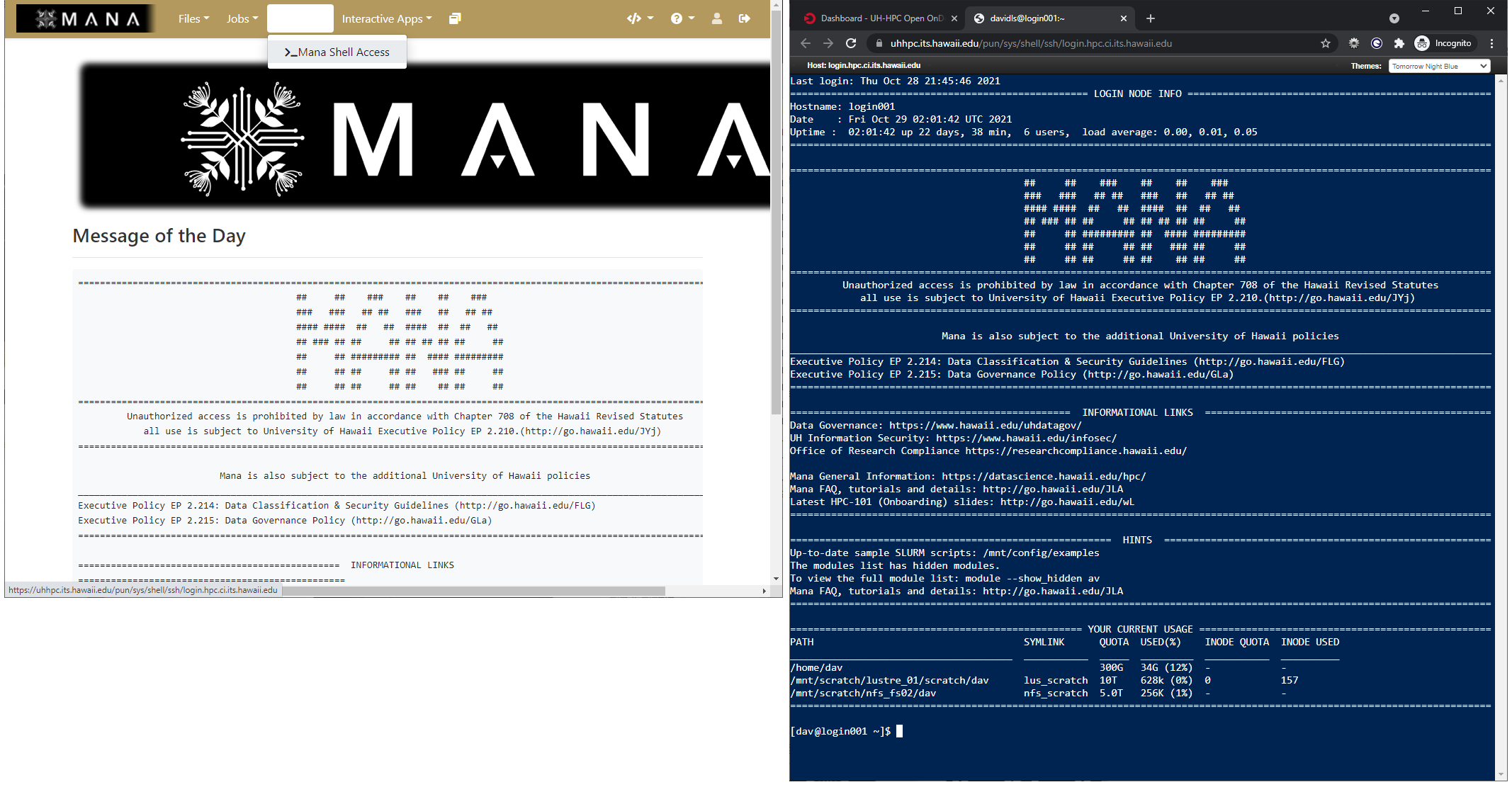
The first step in using a cluster is to establish a connection from our laptop to the cluster. When we are sitting at a computer (or standing, or holding it in our hands or on our wrists), we have come to expect a visual display with icons, widgets, and perhaps some windows or applications: a graphical user interface, or GUI. Since HPC systems are remote resources that we connect to over often slow or laggy interfaces (WiFi and Virtual private networks (VPN)s especially), it is more practical to use a command-line interface, or CLI, in which commands and results are transmitted via text, only. Anything other than text (images, for example) must be written to disk and opened with a separate program.

If you have ever opened the Windows Command Prompt or macOS Terminal, you have seen a CLI. If you have already taken a Carpentries’ course on the UNIX Shell or Version Control, you have used the CLI. The only leap to be made here is to open a CLI on a remote machine, while taking some precautions so that other folks on the network can’t see (or change) the commands you’re running or the results the remote machine sends back. These days, we use the Secure SHell protocol (or SSH) to open an encrypted network connection between two machines, allowing you to send & receive text and data without having to worry about prying eyes.

Traditional HPC system access using Secure Shell (SSH)

Most modern computers have a built in SSH client to their terminal. Alternative clients exist, primarily for windows or add-ons to web browsers, but they all operate in a similar manner. SSH clients are usually command-line tools, where you provide the remote machine address as the only required argument. If your username on the remote system differs from what you use locally, you must provide that as well. If your SSH client has a graphical front-end, such as PuTTY, MobaXterm, you will set these arguments before clicking “connect.” From the terminal, you’ll write something like ssh userName@hostname, where the “@” symbol is used to separate the two parts of a single argument.

Example of ssh on the Linux command line, Mac OS terminal and windows 10 terminal

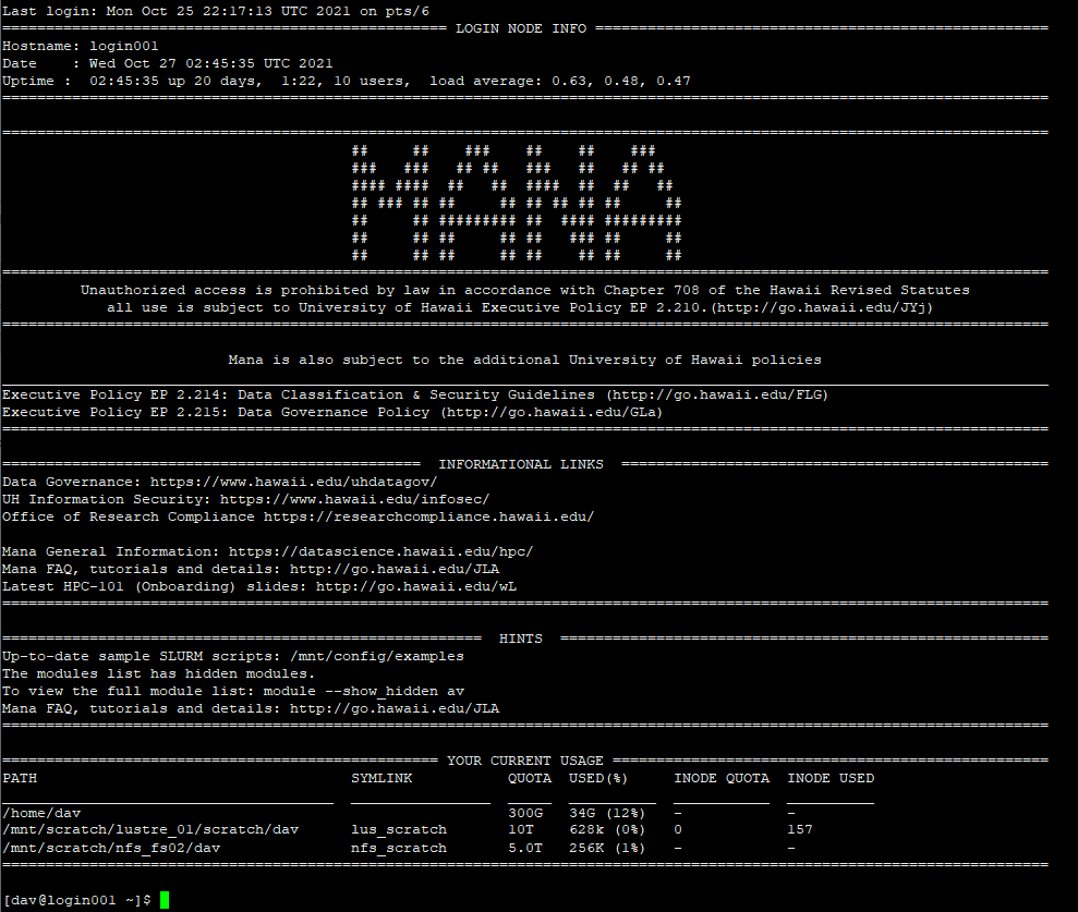
ssh dav@mana.its.hawaii.edu

Take note

You may be asked for your password. Watch out: the characters you type after the password prompt are not displayed on the screen. Normal output will resume once you press Enter.

Open OnDemand - An alternative to using SSH

While, SSH is a common method to connect to remote systems (HPC or even servers), tools that provide the same functionality and more exist. One such tool is Open OnDemand (OOD).

Learn more about Open OnDemand

Created by Ohio Supercomputer Center, U. of Buffalo CCR, and Virginia Tech and development funded by National Science Foundation under grant numbers 1534949 and 1835725. Learn more about Open OnDemand

Features of Open OnDemand

Open OnDemand works with a web browser making it possible to connect to an HPC system with almost any device. It has built in functionality for file browsing, uploading and downloading smaller files, text editing, SSH terminal, and submitting interactive applications such as a remote desktop on a compute node, Jupyter Lab and Rstudio.

Interactive applications at other institutions

Various other interactive applications have been made for Open OnDemand but are not available by default. See here for a list of known interact appilications.

Browser choice and using an incognito or private browsing window

While almost any modern browser should work with Open OnDemand, the developers recommend google chrome as it has the widest support for the tools used to create Open OnDemand. browser requirements

For security it is recommend you use a private browsing window with Open OnDemand as this allows you completely log out by just simplying closing the browser window. While logout does exist in Open OnDemand, it may not work as expected and really keep you logged in even after hitting logout.

Login to Mana using Open onDemand

• Open up your web browser and start a private browsing window. Now, connect to the instance of Open OnDemand used with Mana by pointing your browser at https://mana.its.hawaii.edu.

File browsing and editing

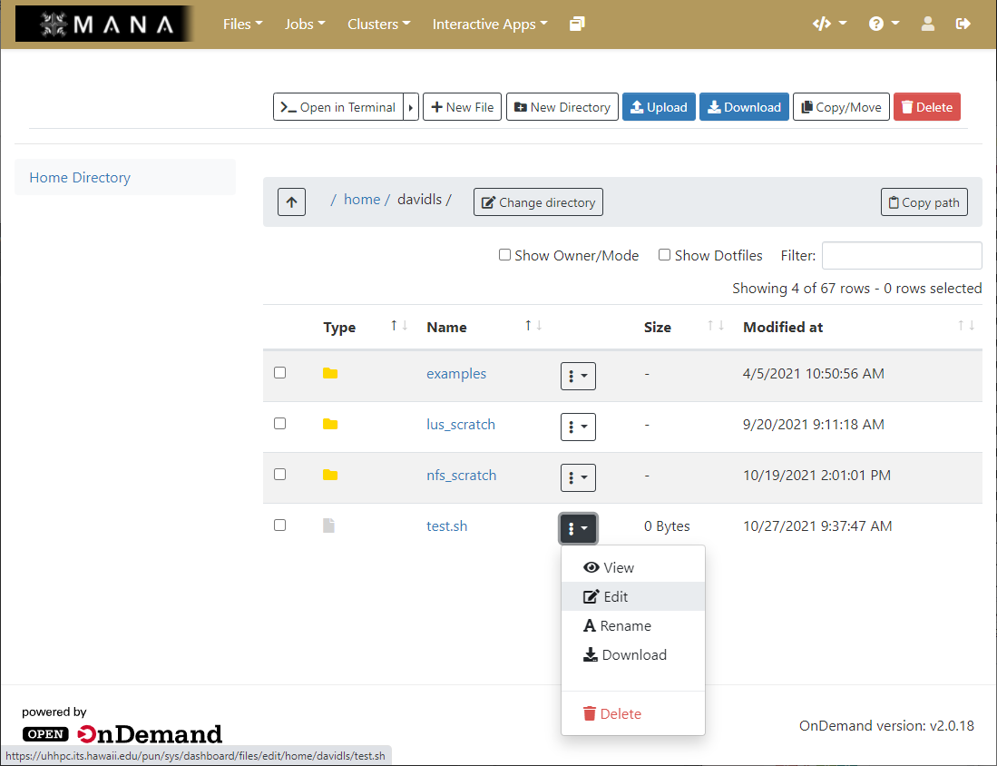
The file browser allows you to perform directory manipulation, create new files, upload and download files without having to know the command line. The file browser can even has the ability to do text editing on files which is useful if you are not familiar with a command line text editor.

Command line text editors

Common text editors you find on HPC systems or linx systems include:

• Vi/Vim
• Emacs
• nano Of the three, nano is the simplest to use

Terminal in the browser

As Open OnDemand doesn’t really replace the traditional commandline/SSH access method to HPC systems, and instead makes the use of certain applications simpler, it still provides a way to bring up a commandline on an HPC system within your web browser.

Interactive applications

While Open OnDemand can allow you to access HPC systems using the terminal, it also has the ability to expand the ways and HPC can be easily used though allowing the use of interactive applications that many have come to depend on.

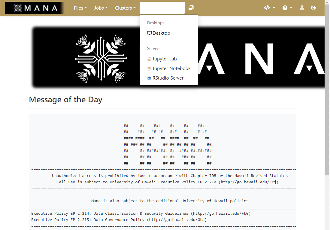
Each application has a form which you use to define the resources your job requires so that Open OnDemand can submit it on your behalf. It also has the ability to email you once your job starts as not all jobs will begin immediately.

Finally, when a job begins, it presents you with a button you can click to start up your interactive application and use it within your browser.

Material used and modfied from the “Introduction to High-Performance Computing” Incubator workshop.

Key Points

• SSH is the traditional method of connecting to HPC systems

• Alternative tools like Open OnDemand exist to enhance the utility of and simplify the access to an HPC system

Deep learning CPU vs GPU

Overview

Teaching: 40 min
Exercises: 10 min

Questions

• How does the performance of GPU compare with that of CPU?

• How to use Mana to do Machine Learning research?

• How to ask for computing resources?

Objectives

• Do a basic Deep Learning tutorial on Mana

Jupyter Lab as an Interactive Application in Open OnDemand

As we previously saw, Open OnDemand allows us to use interactive applications, one of which is Juypter Lab.

The form is used to specify what resources you want, which are then placed into a queue with other waiting jobs and will start to run your job as soon as the resources requested are available.

Under the hood

The Open On Demand form for interactive applications defines a job script and passes it to the HPC systems job scheduler, taking the burden of how to start the application on the HPC system and how to write a job script that the job scheduler can understand off of the user.

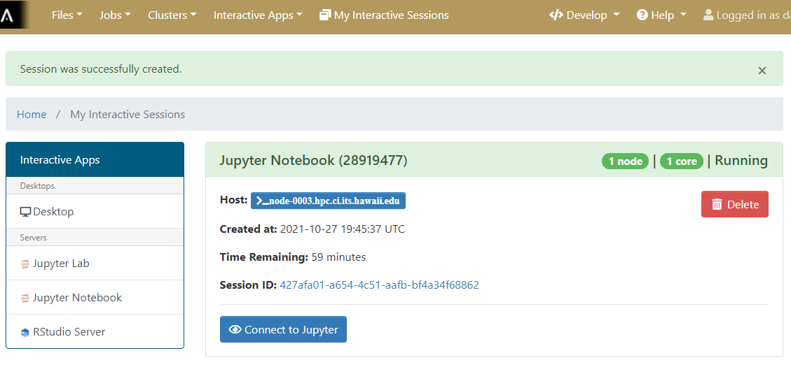
Starting an Interactive session of Jupyter Lab and Open Jyupyter Lab

As we will be working in Jupyter Lab to explore some concepts when working with HPC systems and deep learning your challenge is to start an interactive application of Jupyter Lab with the following parameters

• Partition: workshop
• Number of hours: 3
• Number of Nodes: 1
• Number of Tasks per Node: 1
• Number of cores per task: 4
• GB of Ram: 24 GB
• Number of GPUs requested: 1
• GPU Type: Any

Once the interactive session is running Connect to the jupyter session by click the “Connect to Jupyter” button.

Solution

Why use Jupyter?

For python based data science and machine learning applications, Jupyter notebook is a great platform because:

1. you can store your data, code, do visualizations, equations, text, outputs all in one place,
2. you can easily share your work easily in different formats like JSON, PDF, html,
3. it supports more than 40 programming languages, can switch between differnt environments and has an interactive output,
4. can easily edit the code and re-run it without affecting other sections.

Jupyter Lab vs Jupyter Notebook

Jupyter notebook allows you to access ipython notebooks only (.ipynb files), i.e. it will create a computational environment which stores your code, results, plots, texts etc. And here you can work in only one of your environments. But Jupyter Lab gives a better user interface along with all the facilties provided by the notebook. It is a flexible, web based application with a modular structure where one can access python files (.py), ipython notebooks, html or markdown files, access file browser (to upload, download, copy, rename, delete files), work with multiple Jupyter notebooks and environments, all in the same window.

How does JupyterLab work?

You write your code or plain text in rectangular “cells” and the browser then passes it to the back-end “kernel”, which runs your code and returns output.

File extensions and content

.ipynb file is a python notebook which stores code, text, markdown, plots, results in a specific format but .py file is a python file which only stores code and plain text (like comments etc).

How to access and install softwares and modules on a cluster?

Using a package manager

Working with Python requires one to have different packages installed with a specific version which gets updated once in a while. On Mana, there are software packages already installed on the cluster which one can use to install the required libraries, softwares and can even choose which version to install. You can use following commands to see what modules are available on the cluster or which ones are already loaded or to load a specific module in your environment:

  module avail
  module list 
  module load <MODULE_NAME>

So what is an environment then?

Sometimes different applications require different versions of the Python packages than the one you’ve been using and this is where a Python environment comes in handy.
An environment (or a conda environment specifically, which we’ll discuss later) is a directory, specific or isolated to a project, that contains a specific collection of python packages and their different versions that you have installed. There are 2 most popular tools to set up yur environment:

1. Pip: a tool to install Python software packages only.

2. Anaconda (or Conda): cross platform package and environment manager which lets you access C, C++ libraries, R package for scientific computing along with Python.

Note

Packages contains all the files you need for the modules it supplies

Anaconda

This is a popular package manager in scientific computing which handles the Python and R programming language related dependencies rather easily. It is preferred more because:

• it has a clear directory structure which is easy to understand,
• it allows you to install softwares written in any programming language,
• it gives you a flexibility to create different environments with different software versions (and can install pip packages as well),
• one can use both CLI and GUI.

Environment isloation

If you try to access a library with different version based on your project, pip may throw an error. To create isolated environments you can use virtual environment (venv) with pip.

Environment setup

• Create a conda environment

module load lang/Anaconda3
conda create --name tf2
source activate tf2

• Install relevant libraries

conda install tensorflow-gpu matplotlib tensorflow keras

Difference between conda environment and kernel

Although we created a conda environment, the Jupyter notebook still cannot access it because “conda” is the directory that contains all the installed conda packages but it is the “kernel” that runs the user’s code and can use and access different conda environments, if required. A kernel is the computational engine that executes the code contained in Jupyter notebook or it is the interface which tells Jupyter notebook which kernel it should use to access the packages and softwares.

• Let’s create a python kernel

conda install ipykernel
python -m ipykernel install --user --name tf2 --display-name tf2

Deep Learning Tutorial

This is a basic image classification tutorial from CIFAR-10 dataset using tensorflow.

Tensorflow

It is an open source software used in machine learning particularly for training neural networks. We’ll define our model using ‘Keras’- a high level API which acts as an interface between tensorflow and python and makes it easy to build and train models. You can read more about it here.

CIFAR-10 dataset

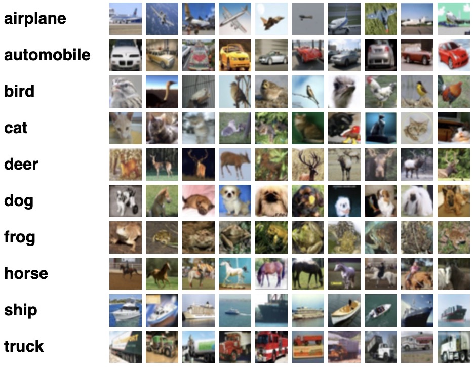
CIFAR-10 is a common dataset used for machine learning and computer vision research. It is a subset of 80 million tiny image dataset and consists of 60,000 images. The images are labelled with 10 different classes. So each class has 5000 training images and 1000 test images. Each row represents a color image of 32 x 32 pixels with 3 channels (RGB).

Basic workflow of Machine Learning

1. Collect the data
2. Pre-process the data
3. Define a model
4. Train the model
5. Evaluate/test the model
6. Improve your model

Working with Cifar-10 dataset

• Import all the relevant libraries

import numpy as np
import matplotlib.pyplot as plt

import tensorflow as tf
import h5py
import keras
from keras.datasets import cifar10
from tensorflow.keras.models import Sequential
from tensorflow.keras.layers import Dense, Conv2D, Flatten, MaxPooling2D, Input, InputLayer, Dropout
import keras.layers.merge as merge
from keras.layers.merge import Concatenate
from tensorflow.keras.utils import to_categorical
from tensorflow.keras.optimizers import SGD, Adam

%matplotlib inline

• Check for CPU and GPU

How to check if you’re using GPU ?

tf.config.list_physical_devices('GPU')

Now, how would you check for CPU ?

Solution

tf.config.list_physical_devices('CPU')

Is GPU necessary for machine learning?

No, machine learning algorithms can be deployed using CPU or GPU, depending on the applications. They both have their distinct properties and which one would be best for your application depends on factors like: speed, power usage and cost. CPUs are more general purposed processors, are cheaper and provide a gateway for data to travel from source to GPU cores. But GPU have an advantage to do parallel computing when dealing with large datasets, complex neural network models. The difference between the two lies in basic features of a processor i.e. cache, clock speed, power consumption, bandwidth and number of cores. Read more that here.

• Load the data and analyze its shape

(x_train, y_train), (x_valid, y_valid) = cifar10.load_data()
nb_classes = 10
class_names = ['airplane', 'automobile', 'bird', 'cat', 'deer', 'dog', 'frog', 'horse', 'ship', 'truck']
print('Train: X=%s, y=%s' % (x_train.shape, y_train.shape))
print('Test: X=%s, y=%s' % (x_valid.shape, y_valid.shape))
print('number of classes= %s' %len(set(y_train.flatten())))
print(type(x_train))

Solution

Train: X=(50000, 32, 32, 3), y=(50000, 1)
Test: X=(10000, 32, 32, 3), y=(10000, 1)
number of classes= 10
<class 'numpy.ndarray'>

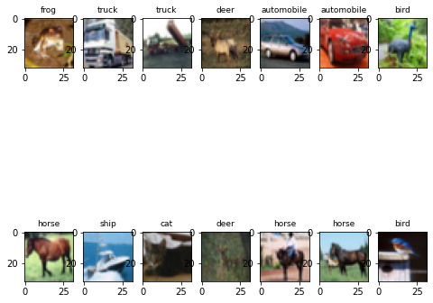
• Plot some examples

plt.figure(figsize=(8, 8)) 
for i in range(2*7):
    # define subplot
    plt.subplot(2, 7, i+1)
    plt.imshow(x_train [i])
    class_index = np.argmax(to_categorical(y_train[i], 10))
    plt.title(class_names[class_index], fontsize=9)

Solution

• Convert data to HDF5 format

with h5py.File('dataset_cifar10.hdf5', 'w') as hf:
    dset_x_train = hf.create_dataset('x_train', data=x_train, shape=(50000, 32, 32, 3), compression='gzip', chunks=True)
    dset_y_train = hf.create_dataset('y_train', data=y_train, shape=(50000, 1), compression='gzip', chunks=True)
    dset_x_test = hf.create_dataset('x_valid', data=x_valid, shape=(10000, 32, 32, 3), compression='gzip', chunks=True)
    dset_y_test = hf.create_dataset('y_valid', data=y_valid, shape=(10000, 1), compression='gzip', chunks=True)

What is HDF5 file?

HDF5 file format is a binary data format which is mainly used to store large, heterogenous files. It provides fast, parallel I/O processing. You can learn more about it here and here.

• Define the model

model = tf.keras.Sequential()
model.add(InputLayer(input_shape=[32, 32, 3]))

model.add(Conv2D(filters=32, kernel_size=3, padding='same', activation='relu'))
model.add(MaxPooling2D(pool_size=[2,2], strides=[2, 2], padding='same'))

model.add(Conv2D(filters=64, kernel_size=3, padding='same', activation='relu'))
model.add(MaxPooling2D(pool_size=[2,2], strides=[2, 2], padding='same'))

model.add(Conv2D(filters=128, kernel_size=3, padding='same', activation='relu'))
model.add(MaxPooling2D(pool_size=[2,2], strides=[2, 2], padding='same'))

model.add(Conv2D(filters=256, kernel_size=3, padding='same', activation='relu'))
model.add(MaxPooling2D(pool_size=[2,2], strides=[2, 2], padding='same'))

model.add(Flatten())

model.add(Dense(256, activation='relu'))
model.add(Dropout(0.2))

model.add(Dense(512, activation='relu'))
model.add(Dropout(0.2))

model.add(Dense(10, activation='softmax'))

model.summary()

• Define the data generator

class DataGenerator(tf.keras.utils.Sequence):
   
    def __init__(self, batch_size, test=False, shuffle=True):
       
        PATH_TO_FILE = 'dataset_cifar10.hdf5'
       
        self.hf = h5py.File(PATH_TO_FILE, 'r')         
        self.batch_size = batch_size
        self.test = test
        self.shuffle = shuffle
        self.on_epoch_end()

    def __del__(self):
        self.hf.close()
       
    def __len__(self):
        return int(np.ceil(len(self.indices) / self.batch_size))

    def __getitem__(self, idx):
        start = self.batch_size * idx
        stop = self.batch_size * (idx+1)
       
        if self.test:
            x = self.hf['x_valid'][start:stop, ...]
            batch_x = np.array(x).astype('float32') / 255.0
            y = self.hf['y_valid'][start:stop]
            batch_y = to_categorical(np.array(y), 10)
        else:
            x = self.hf['x_train'][start:stop, ...]
            batch_x = np.array(x).astype('float32') / 255.0
            y = self.hf['y_train'][start:stop]
            batch_y = to_categorical(np.array(y), 10)

        return batch_x, batch_y

    def on_epoch_end(self):
        if self.test:
            self.indices = np.arange(self.hf['x_valid'][:].shape[0])
        else:
            self.indices = np.arange(self.hf['x_train'][:].shape[0])
           
        if self.shuffle:
            np.random.shuffle(self.indices)

• Generate batches of data for training and validation dataset

batchsize  = 250 
data_train = DataGenerator(batch_size=batchsize)
data_valid = DataGenerator(batch_size=batchsize, test=True, shuffle=False)

• First, let’s train the model using CPU

with tf.device('/device:CPU:0'):
    history = model.fit(data_train,epochs=10,
                        verbose=1, validation_data=data_valid)

• Now, lets try with GPU to compare its performance with CPU

from tensorflow.keras.models import clone_model
new_model = clone_model(model)
opt = keras.optimizers.Adam(learning_rate=0.001)
new_model.compile(optimizer=opt, loss='categorical_crossentropy', metrics=['accuracy'])  
                        
##### train the new model with GPU #####

Solution

with tf.device('/device:GPU:0'):
    new_history = new_model.fit(data_train,epochs=10,
                                verbose=1, validation_data=data_valid)

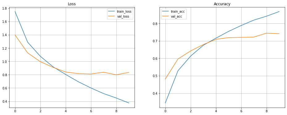
• Plotting the losses and accuracy for training and validation set

fig, axes = plt.subplots(1,2, figsize=[16, 6])
axes[0].plot(history.history['loss'], label='train_loss')
axes[0].plot(history.history['val_loss'], label='val_loss')
axes[0].set_title('Loss')
axes[0].legend()
axes[0].grid()
axes[1].plot(history.history['accuracy'], label='train_acc')
axes[1].plot(history.history['val_accuracy'], label='val_acc')
axes[1].set_title('Accuracy')
axes[1].legend()
axes[1].grid()

Solution

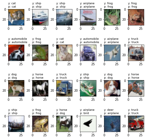
• Evaluate the model and make predictions

x = x_valid.astype('float32') / 255.0
y = to_categorical(y_valid, 10)
score = new_model.evaluate(x, y, verbose=0)
print('Test cross-entropy loss: %0.5f' % score[0])
print('Test accuracy: %0.2f' % score[1])

y_pred = new_model.predict_classes(x)

• Plot the predictions

plt.figure(figsize=(8, 8)) 
for i in range(20):
    plt.subplot(4, 5, i+1)
    plt.imshow(x[i].reshape(32,32,3))
    index1 = np.argmax(y[i])
    plt.title("y: %s\np: %s" % (class_names[index1], class_names[y_pred[i]]), fontsize=9, loc='left')
    plt.subplots_adjust(wspace=0.5, hspace=0.4)

Solution

Other resources to do Machine Learning

• You can use Google Colab which uses Jupyter notebooks too but on Google server. Here you can get free limited compute resources (even GPU) and upgrade your account (for TPU) if you want more. The code usually runs on Google servers on cloud and is connected to your google account so all your projects will be saved in your Google Drive.
• Microsoft Azure notebook is similar to Google Colab with cloud sharing functionality but provides more memory.
• Kaggle
• Amazon Sage Maker

Discuss

Why would you need an HPC cluster over your personal computer?

Key Points

• Open On Demand requires you have a strong, stable internet connection whereas SSH can work with weak connections too.

• JupyterLab is a more common platform for data science research but there are other IDE (Integrated Development Environment softwares) like PyCharm, Spyder, RMarkdown too.

• Using multiple GPUs won’t improve the performance of your machine learning model. It only helps for a very complex computation or large models.

Staging and File System Choice

Overview

Teaching: 20 min
Exercises: 20 min

Questions

• What is a file system?

• What is a distributed file system?

• How do you optimize file system on Mana?

Objectives

• Understand general file system and distributed file system concepts.

• Being able to stage files on Mana lustre scratch.

What is a file system?

The term file system is ubiquitous among operating systems. At some point in time, you may have had to format a USB flash drive (SD card, memory stick) and may have to choose between different file systems such as FAT32 or NTFS (on a Windows OS), exFat or Mac OS Extended (on a Mac).

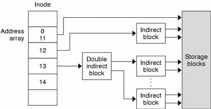
File systems are ways in which operating systems organize data (i.e. documents, movies, music) on storage devices. From the storage device hardware perspective, data is represented as a sequence of blocks of bytes, however that by itself isn’t useful to regular users. Regular users mostly care about file and directory level abstraction and rarely work with blocks of bytes! Luckily, the file system under the hood handles the organization and locating logic of these blocks of bytes for the users so that you can run your favorite commands (e.g., ls) and applications. For example in a Linux file system, “file” information is stored in an inode table (illustrated in figure above) as sort of a lookup table for locating corresponding blocks of a particular file on disk. Located blocks are combined together to form a single file which the end user can work with.

What is a distributed file system?

On a cluster, blocks of data that make up a single file are distributed among network attached storage or NAS devices. Similar principles apply here, the goal of a cluster file system is still to organize and locate blocks of data (but across network!) and present them to the end user as one contiguous file. One main benefit of stringing storage devices together into a network connected cluster is to increase storage capacity beyond what a single computer can have. Imagine working with 100 TB files on your laptop. Of course, the storage can be shared with different cluster users further increasing utilization of these storage devices.

On Mana, the two main supported file systems are Network File System (NFS) and Lustre. Mana users have two special folders called lus_scratch and nfs_scratch where they can temporarily store data on the cluster. Note that the scratch folders will be purged after some period of time, please save your important files into your home directory.

Locate Lustre and NFS File System Scratch On Mana

Let’s locate our lustre and nfs scratch folder. First create a new cell in our Jupyter Lab Notebook after the first cell Paste the code into the cell and run. The pwd command will print where you are in the directory tree and it should be something like “/home/username The ls command will print files and directory that are available in your home/username directory. You should see “lus_scratch” and “nfs_scratch” listed in the print out. Note that the ‘!’ symbol below allows us to execute terminal commands in our Jupyter Lab Notebook cell.

!pwd
!ls

Lustre File System.

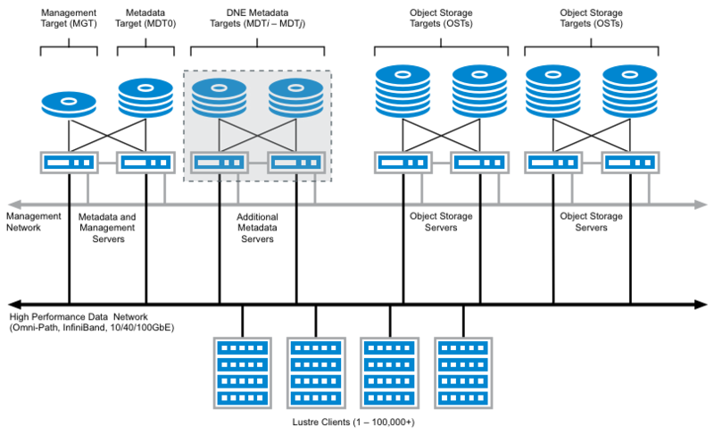
Lustre is a parallel distributed file system, where file operations are distributed across multiple file system servers. In Lustre, storage is divided among multiple servers allowing for ease of scalability and fault tolerance. This file system is great for high speed read/write performance.

NFS File System

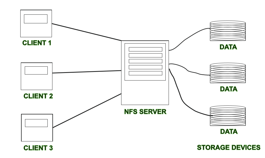
NFS is a single server distributed file system where file operations are not parallel across servers but a single server serves requests to the cluster. NFS is an older technology and has the advantage of having gone through the test of time and is trusted among cluster architects.

Choosing the Right File System For Performance

Depending on the user’s need, different file systems are optimized for different purposes. One may be optimized for random access speed, one with error correcting capability, or one with high redundancy to prevent loss of data. For this workshop, we will focus on disk random access speed Mana cluster.

On Mana we have 3 locations for file storage: “home/user”, “lus_scratch”, and “nfs_scratch” folders available to us. On Mana, our “home/user” directory resides on an NFS file system server. Though “home/user” is great for storing our files on the cluster, it’s serverly lacking in read/write performance. For the best performance (read/write speed) we will mostly want to use “lus_scratch”. As discussed above, the reason is because Lustre file system distributes workload accross multiple meta servers, while NFS is a single server file system. In addition, Mana Lustre file system is configured with solid state drives while NFS file system is configured with hardrives, improving Mana lustre file system read/write speed further.

Solid State Drive vs. Hardrive Performance

Solid state drives can read up to 10 times faster and writes up to 20 times faster than hard disk drive. You can read more about it here.

List Usage Information

On Mana, there’s a command that lists disk usage on the cluster. Create a new cell below our previous block. Paste the code into the cell and run. You should see a table that lists disk space used and remaining space.

!usage

Simulating Read/Write Load

Let’s compare read/write speed between the 2 file systems. In new cells, define a write function that simulates writes to our file system and define a read function that simulates read from our file systems. Note that internally, file write operation is buffered to memory, this is the reason why we need to flush our buffer so that actual writes to disk happens.

def write_large_file(path):
   with open(path, 'w') as f:
       for i in range(1000000):
           f.write(str(i))
           f.flush()
def read_large_file(path):
   with open(path, 'r') as f:
       for i in range(1000000):
           f.read(1)

Timing Read/Write Operations

Now that we have defined our read/write functions, let’s profile them. In new cells, call our read / write functions from our “lus_scratch” directory. Similarly call our read/write functions from our “home” directory (remember that home directory resides in Mana NFS file system servers). To time the cells, we can call “%%time” at the beggining of our cells. This is a special command in Jupyter Lab Notebook that allows us to time execution time of a cell.

%%time
write_large_file("./lus_scratch/large_file.txt")

%%time
read_large_file("./lus_scratch/large_file.txt")

%%time
write_large_file("./large_file.txt")

%%time
read_large_file("./large_file.txt")

Read Speed Improvement Performance

From the challenge, we may notice a very small improvement in read performance. This is most likely due to the fact that we do sequential reads (read more about that here) and also the fact the created file is too small to show the difference in improvement.

Optimizing Our Deep Learning Code

We can optimize our Deep Learning Jupyter Lab Notebook further by utilizing “lus_scratch” folder. Instead of reading and writing training data from our home directory, we’re going to instead work from the “lus_scratch” directory.

Stage Training Files

We will now make a copy of the training data into the “lus_scratch” directory. Create a new cell in our Jupyter Lab Notebook. Paste the code below into the cell. Update the path so that the data is save into our “lus_scratch” directory. You should see a print out of the with “dataset_cifar10.hdf5”.

# Stage files onto luster directory.
with h5py.File('./lus_scratch/dataset_cifar10.hdf5', 'w') as hf:
   dset_x_train = hf.create_dataset('x_train', data=x_train, shape=(50000, 32, 32, 3), compression='gzip', chunks=True)
   dset_y_train = hf.create_dataset('y_train', data=y_train, shape=(50000, 1), compression='gzip', chunks=True)
   dset_x_test = hf.create_dataset('x_valid', data=x_valid, shape=(10000, 32, 32, 3), compression='gzip', chunks=True)
   dset_y_test = hf.create_dataset('y_valid', data=y_valid, shape=(10000, 1), compression='gzip', chunks=True)
!ls "./lus_scratch/"

Update Data Generator File Path

Now that we have successfully staged our training data to the “lus_scratch” directory, let us now update the data path for our data generator. Find where the data is loaded, the code in the cell should look like the code below. Once the cell is updated, run the cell.

filename = "./lus_scratch/dataset_cifar10.hdf5"
batchsize  = 250 
data_train_lus = DataGenerator(filename, batch_size=batchsize, test=False)
data_valid_lus = DataGenerator(filename, batch_size=batchsize, test=True, shuffle=False)

Rerun The Model With The Updated Data Generator

Let’s rerun our model with the new data generator objects. Use the GPU version of the training code similiar to below. Run training step of the model. Compare the training time. Note: As we’ve seen previously, both file systems are comparable in read speed for small data sets. Here, we may not see a huge difference since we’re mostly performing read. With bigger data sets, such as “cifar100” data set, differences in read speed will be more noticable.

from tensorflow.keras.models import clone_model
new_model = clone_model(model)
opt = keras.optimizers.Adam(learning_rate=0.001)
new_model.compile(optimizer=opt, loss='categorical_crossentropy', metrics=['accuracy'])
with tf.device('/device:GPU:0'):
   new_history = new_model.fit(data_train_lus, epochs=10,
                                verbose=1, validation_data=data_valid_lus)

Key Points

• File system is a way in which operating systems organize data on storage devices.

• Distributed file system organizes data accross network attached storage devices.

• Distributed file system has the advantage of supporting larger scale storage capacity.

• Mana supports lustre and NFS file systems.

• Lustre on Mana is setup with solid state drives.

• NFS on Mana is setup with spinning drives.