Deep learning CPU vs GPU

Overview

Teaching: 40 min
Exercises: 10 min

Questions

How does the performance of GPU compare with that of CPU?

How to use Mana to do Machine Learning research?

How to ask for computing resources?

Objectives

Do a basic Deep Learning tutorial on Mana

Jupyter Lab as an Interactive Application in Open OnDemand

As we previously saw, Open OnDemand allows us to use interactive applications, one of which is Juypter Lab.

/High_Performance_Computing/Connect%20to%20cluster

The form is used to specify what resources you want, which are then placed into a queue with other waiting jobs and will start to run your job as soon as the resources requested are available.

Under the hood

The Open On Demand form for interactive applications defines a job script and passes it to the HPC systems job scheduler, taking the burden of how to start the application on the HPC system and how to write a job script that the job scheduler can understand off of the user.

Starting an Interactive session of Jupyter Lab and Open Jyupyter Lab

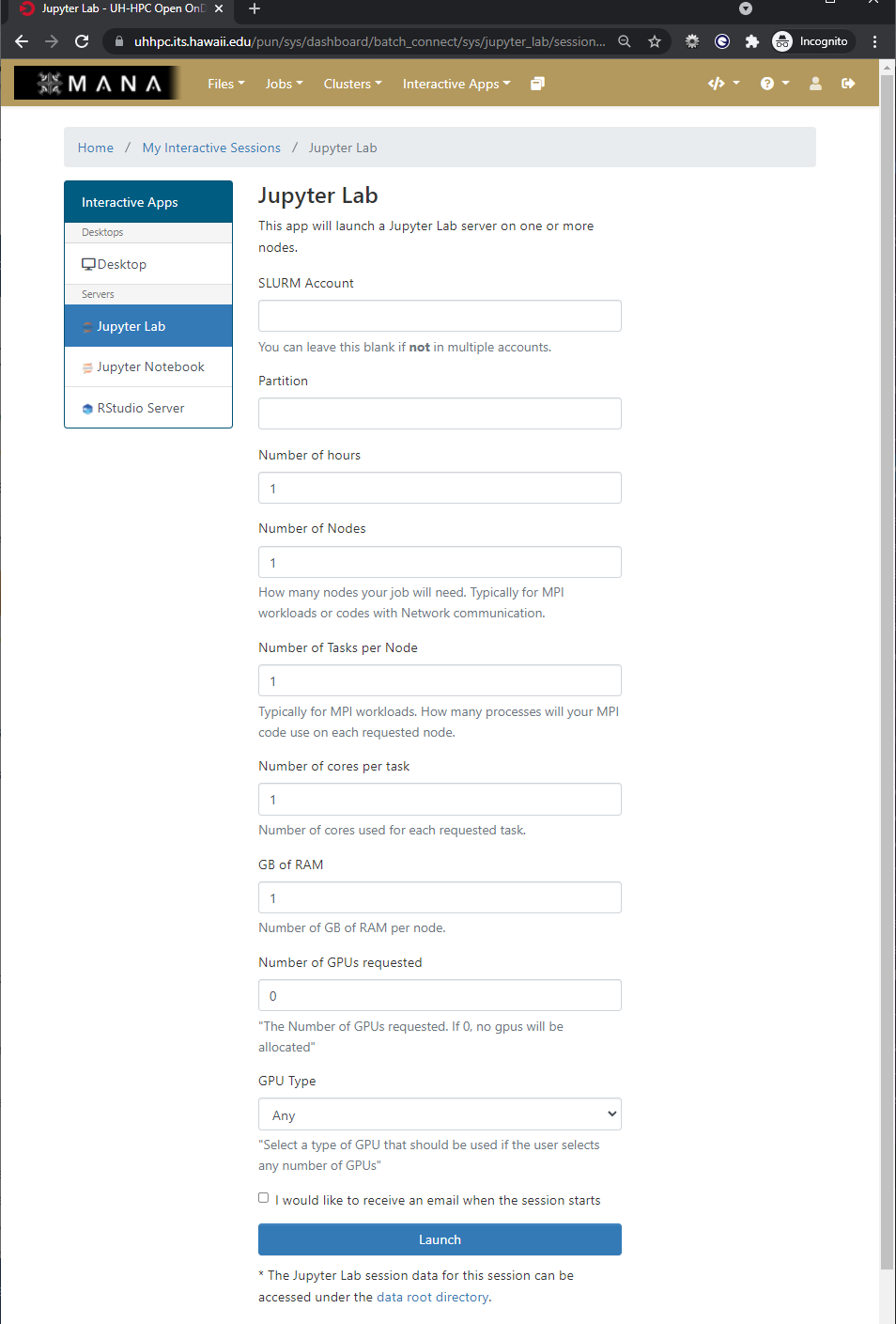
As we will be working in Jupyter Lab to explore some concepts when working with HPC systems and deep learning your challenge is to start an interactive application of Jupyter Lab with the following parameters

Partition: workshop

Number of hours: 3

Number of Nodes: 1

Number of Tasks per Node: 1

Number of cores per task: 4

GB of Ram: 24 GB

Number of GPUs requested: 1

GPU Type: Any

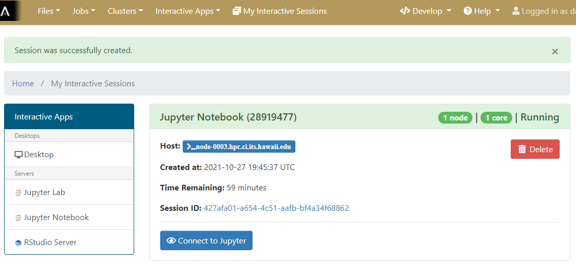
Once the interactive session is running Connect to the jupyter session by click the “Connect to Jupyter” button.

Solution

Why use Jupyter?

For python based data science and machine learning applications, Jupyter notebook is a great platform because:

you can store your data, code, do visualizations, equations, text, outputs all in one place,
you can easily share your work easily in different formats like JSON, PDF, html,
it supports more than 40 programming languages, can switch between differnt environments and has an interactive output,
can easily edit the code and re-run it without affecting other sections.

Jupyter Lab vs Jupyter Notebook

Jupyter notebook allows you to access ipython notebooks only (.ipynb files), i.e. it will create a computational environment which stores your code, results, plots, texts etc. And here you can work in only one of your environments. But Jupyter Lab gives a better user interface along with all the facilties provided by the notebook. It is a flexible, web based application with a modular structure where one can access python files (.py), ipython notebooks, html or markdown files, access file browser (to upload, download, copy, rename, delete files), work with multiple Jupyter notebooks and environments, all in the same window.

How does JupyterLab work?

You write your code or plain text in rectangular “cells” and the browser then passes it to the back-end “kernel”, which runs your code and returns output.

File extensions and content

.ipynb file is a python notebook which stores code, text, markdown, plots, results in a specific format but .py file is a python file which only stores code and plain text (like comments etc).

How to access and install softwares and modules on a cluster?

Using a package manager

Working with Python requires one to have different packages installed with a specific version which gets updated once in a while. On Mana, there are software packages already installed on the cluster which one can use to install the required libraries, softwares and can even choose which version to install. You can use following commands to see what modules are available on the cluster or which ones are already loaded or to load a specific module in your environment:

  module avail
  module list 
  module load <MODULE_NAME>

So what is an environment then?

Sometimes different applications require different versions of the Python packages than the one you’ve been using and this is where a Python environment comes in handy.
An environment (or a conda environment specifically, which we’ll discuss later) is a directory, specific or isolated to a project, that contains a specific collection of python packages and their different versions that you have installed. There are 2 most popular tools to set up yur environment:

Pip: a tool to install Python software packages only.
Anaconda (or Conda): cross platform package and environment manager which lets you access C, C++ libraries, R package for scientific computing along with Python.

Note

Packages contains all the files you need for the modules it supplies

Anaconda

This is a popular package manager in scientific computing which handles the Python and R programming language related dependencies rather easily. It is preferred more because:

it has a clear directory structure which is easy to understand,
it allows you to install softwares written in any programming language,
it gives you a flexibility to create different environments with different software versions (and can install pip packages as well),
one can use both CLI and GUI.

/High_Performance_Computing/Anaconda%20+%20Python

Environment isloation

If you try to access a library with different version based on your project, pip may throw an error. To create isolated environments you can use virtual environment (venv) with pip.

Environment setup

Create a conda environment
module load lang/Anaconda3
conda create --name tf2
source activate tf2
Install relevant libraries
conda install tensorflow-gpu matplotlib tensorflow keras
Difference between conda environment and kernel

Although we created a conda environment, the Jupyter notebook still cannot access it because “conda” is the directory that contains all the installed conda packages but it is the “kernel” that runs the user’s code and can use and access different conda environments, if required. A kernel is the computational engine that executes the code contained in Jupyter notebook or it is the interface which tells Jupyter notebook which kernel it should use to access the packages and softwares.

Let’s create a python kernel
conda install ipykernel
python -m ipykernel install --user --name tf2 --display-name tf2

Deep Learning Tutorial

This is a basic image classification tutorial from CIFAR-10 dataset using tensorflow.

Tensorflow

It is an open source software used in machine learning particularly for training neural networks. We’ll define our model using ‘Keras’- a high level API which acts as an interface between tensorflow and python and makes it easy to build and train models. You can read more about it here.

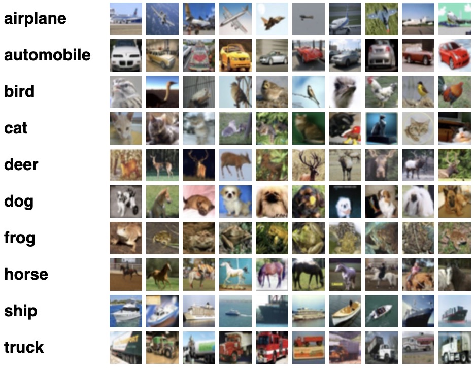
CIFAR-10 dataset

CIFAR-10 is a common dataset used for machine learning and computer vision research. It is a subset of 80 million tiny image dataset and consists of 60,000 images. The images are labelled with 10 different classes. So each class has 5000 training images and 1000 test images. Each row represents a color image of 32 x 32 pixels with 3 channels (RGB).

Basic workflow of Machine Learning

Collect the data
Pre-process the data
Define a model
Train the model
Evaluate/test the model
Improve your model

Working with Cifar-10 dataset

Import all the relevant libraries

import numpy as np
import matplotlib.pyplot as plt

import tensorflow as tf
import h5py
import keras
from keras.datasets import cifar10
from tensorflow.keras.models import Sequential
from tensorflow.keras.layers import Dense, Conv2D, Flatten, MaxPooling2D, Input, InputLayer, Dropout
import keras.layers.merge as merge
from keras.layers.merge import Concatenate
from tensorflow.keras.utils import to_categorical
from tensorflow.keras.optimizers import SGD, Adam

%matplotlib inline

Check for CPU and GPU

How to check if you’re using GPU ?

tf.config.list_physical_devices('GPU')

Now, how would you check for CPU ?

Solution

tf.config.list_physical_devices('CPU')

Is GPU necessary for machine learning?

No, machine learning algorithms can be deployed using CPU or GPU, depending on the applications. They both have their distinct properties and which one would be best for your application depends on factors like: speed, power usage and cost. CPUs are more general purposed processors, are cheaper and provide a gateway for data to travel from source to GPU cores. But GPU have an advantage to do parallel computing when dealing with large datasets, complex neural network models. The difference between the two lies in basic features of a processor i.e. cache, clock speed, power consumption, bandwidth and number of cores. Read more that here.

Load the data and analyze its shape

(x_train, y_train), (x_valid, y_valid) = cifar10.load_data()
nb_classes = 10
class_names = ['airplane', 'automobile', 'bird', 'cat', 'deer', 'dog', 'frog', 'horse', 'ship', 'truck']
print('Train: X=%s, y=%s' % (x_train.shape, y_train.shape))
print('Test: X=%s, y=%s' % (x_valid.shape, y_valid.shape))
print('number of classes= %s' %len(set(y_train.flatten())))
print(type(x_train))

Solution

Train: X=(50000, 32, 32, 3), y=(50000, 1)
Test: X=(10000, 32, 32, 3), y=(10000, 1)
number of classes= 10
<class 'numpy.ndarray'>

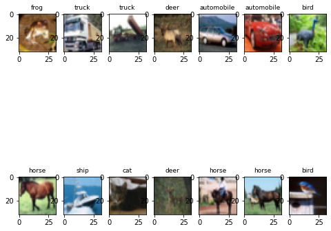
Plot some examples

plt.figure(figsize=(8, 8)) 
for i in range(2*7):
    # define subplot
    plt.subplot(2, 7, i+1)
    plt.imshow(x_train [i])
    class_index = np.argmax(to_categorical(y_train[i], 10))
    plt.title(class_names[class_index], fontsize=9)

Solution

Convert data to HDF5 format

with h5py.File('dataset_cifar10.hdf5', 'w') as hf:
    dset_x_train = hf.create_dataset('x_train', data=x_train, shape=(50000, 32, 32, 3), compression='gzip', chunks=True)
    dset_y_train = hf.create_dataset('y_train', data=y_train, shape=(50000, 1), compression='gzip', chunks=True)
    dset_x_test = hf.create_dataset('x_valid', data=x_valid, shape=(10000, 32, 32, 3), compression='gzip', chunks=True)
    dset_y_test = hf.create_dataset('y_valid', data=y_valid, shape=(10000, 1), compression='gzip', chunks=True)

What is HDF5 file?

HDF5 file format is a binary data format which is mainly used to store large, heterogenous files. It provides fast, parallel I/O processing. You can learn more about it here and here.

Define the model

model = tf.keras.Sequential()
model.add(InputLayer(input_shape=[32, 32, 3]))

model.add(Conv2D(filters=32, kernel_size=3, padding='same', activation='relu'))
model.add(MaxPooling2D(pool_size=[2,2], strides=[2, 2], padding='same'))

model.add(Conv2D(filters=64, kernel_size=3, padding='same', activation='relu'))
model.add(MaxPooling2D(pool_size=[2,2], strides=[2, 2], padding='same'))

model.add(Conv2D(filters=128, kernel_size=3, padding='same', activation='relu'))
model.add(MaxPooling2D(pool_size=[2,2], strides=[2, 2], padding='same'))

model.add(Conv2D(filters=256, kernel_size=3, padding='same', activation='relu'))
model.add(MaxPooling2D(pool_size=[2,2], strides=[2, 2], padding='same'))

model.add(Flatten())

model.add(Dense(256, activation='relu'))
model.add(Dropout(0.2))

model.add(Dense(512, activation='relu'))
model.add(Dropout(0.2))

model.add(Dense(10, activation='softmax'))

model.summary()

Define the data generator

class DataGenerator(tf.keras.utils.Sequence):
   
    def __init__(self, batch_size, test=False, shuffle=True):
       
        PATH_TO_FILE = 'dataset_cifar10.hdf5'
       
        self.hf = h5py.File(PATH_TO_FILE, 'r')         
        self.batch_size = batch_size
        self.test = test
        self.shuffle = shuffle
        self.on_epoch_end()

    def __del__(self):
        self.hf.close()
       
    def __len__(self):
        return int(np.ceil(len(self.indices) / self.batch_size))

    def __getitem__(self, idx):
        start = self.batch_size * idx
        stop = self.batch_size * (idx+1)
       
        if self.test:
            x = self.hf['x_valid'][start:stop, ...]
            batch_x = np.array(x).astype('float32') / 255.0
            y = self.hf['y_valid'][start:stop]
            batch_y = to_categorical(np.array(y), 10)
        else:
            x = self.hf['x_train'][start:stop, ...]
            batch_x = np.array(x).astype('float32') / 255.0
            y = self.hf['y_train'][start:stop]
            batch_y = to_categorical(np.array(y), 10)

        return batch_x, batch_y

    def on_epoch_end(self):
        if self.test:
            self.indices = np.arange(self.hf['x_valid'][:].shape[0])
        else:
            self.indices = np.arange(self.hf['x_train'][:].shape[0])
           
        if self.shuffle:
            np.random.shuffle(self.indices)

Generate batches of data for training and validation dataset

batchsize  = 250 
data_train = DataGenerator(batch_size=batchsize)
data_valid = DataGenerator(batch_size=batchsize, test=True, shuffle=False)

First, let’s train the model using CPU

with tf.device('/device:CPU:0'):
    history = model.fit(data_train,epochs=10,
                        verbose=1, validation_data=data_valid)

Now, lets try with GPU to compare its performance with CPU

from tensorflow.keras.models import clone_model
new_model = clone_model(model)
opt = keras.optimizers.Adam(learning_rate=0.001)
new_model.compile(optimizer=opt, loss='categorical_crossentropy', metrics=['accuracy'])  
                        
##### train the new model with GPU #####

Solution

with tf.device('/device:GPU:0'):
    new_history = new_model.fit(data_train,epochs=10,
                                verbose=1, validation_data=data_valid)

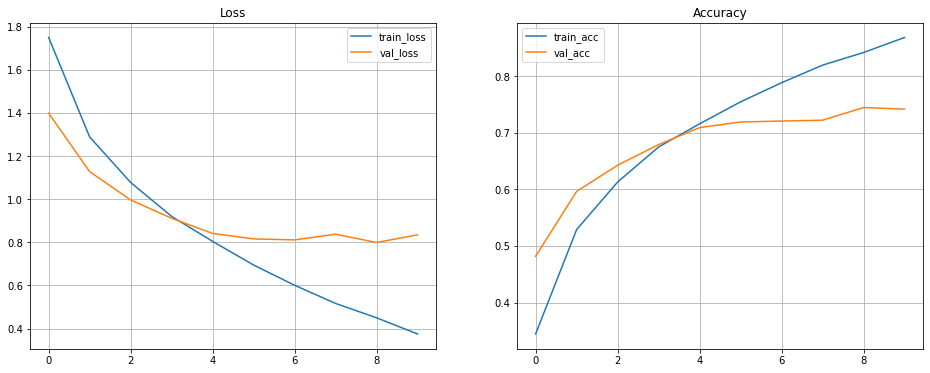
Plotting the losses and accuracy for training and validation set

fig, axes = plt.subplots(1,2, figsize=[16, 6])
axes[0].plot(history.history['loss'], label='train_loss')
axes[0].plot(history.history['val_loss'], label='val_loss')
axes[0].set_title('Loss')
axes[0].legend()
axes[0].grid()
axes[1].plot(history.history['accuracy'], label='train_acc')
axes[1].plot(history.history['val_accuracy'], label='val_acc')
axes[1].set_title('Accuracy')
axes[1].legend()
axes[1].grid()

Solution

Evaluate the model and make predictions

x = x_valid.astype('float32') / 255.0
y = to_categorical(y_valid, 10)
score = new_model.evaluate(x, y, verbose=0)
print('Test cross-entropy loss: %0.5f' % score[0])
print('Test accuracy: %0.2f' % score[1])

y_pred = new_model.predict_classes(x)

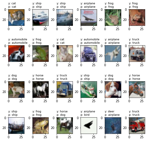
Plot the predictions

plt.figure(figsize=(8, 8)) 
for i in range(20):
    plt.subplot(4, 5, i+1)
    plt.imshow(x[i].reshape(32,32,3))
    index1 = np.argmax(y[i])
    plt.title("y: %s\np: %s" % (class_names[index1], class_names[y_pred[i]]), fontsize=9, loc='left')
    plt.subplots_adjust(wspace=0.5, hspace=0.4)

Solution

Other resources to do Machine Learning

You can use Google Colab which uses Jupyter notebooks too but on Google server. Here you can get free limited compute resources (even GPU) and upgrade your account (for TPU) if you want more. The code usually runs on Google servers on cloud and is connected to your google account so all your projects will be saved in your Google Drive.
Microsoft Azure notebook is similar to Google Colab with cloud sharing functionality but provides more memory.
Kaggle
Amazon Sage Maker

Discuss

Why would you need an HPC cluster over your personal computer?

Key Points

Open On Demand requires you have a strong, stable internet connection whereas SSH can work with weak connections too.

JupyterLab is a more common platform for data science research but there are other IDE (Integrated Development Environment softwares) like PyCharm, Spyder, RMarkdown too.

Using multiple GPUs won’t improve the performance of your machine learning model. It only helps for a very complex computation or large models.

previous episode

High Performance Computing

next episode

Deep learning CPU vs GPU

Overview

Jupyter Lab as an Interactive Application in Open OnDemand

Under the hood

Starting an Interactive session of Jupyter Lab and Open Jyupyter Lab

Solution

Why use Jupyter?

Jupyter Lab vs Jupyter Notebook

How does JupyterLab work?

File extensions and content

How to access and install softwares and modules on a cluster?

Using a package manager

So what is an environment then?

Note

Anaconda

Environment isloation

Environment setup

Difference between conda environment and kernel

Deep Learning Tutorial

Tensorflow

CIFAR-10 dataset

Basic workflow of Machine Learning

Working with Cifar-10 dataset

How to check if you’re using GPU ?

Solution

Is GPU necessary for machine learning?

Solution

Solution

What is HDF5 file?

Solution

Solution

Solution

Other resources to do Machine Learning

Discuss

Key Points

previous episode

next episode