Collaborating and Data Analysis Using HydroShare Workflows
Overview
Teaching: 20 min
Exercises: 2 minQuestions
How do users discover and join an existing research group in HydroShare?
How do users access existing resources and scientific workflows in a group?
How can users use an existing workflow to carry out data analysis?
Objectives
Allow the audience some experience using science gateways and existing workflows for data analysis in a collaborative environment
In the following sections, examples are provided to gain hands-on experience discovering groups and resources of interest, joining a collaborative environment, and performing analysis on data who’s results can be written back to HydroShare to share with others in the group.
More specifically, users will learn the following:
- How to discover and join an existing group of interest
- How to navigate the groups landing page and access its resources
- How to use an existing workflow to carry out some data analysis using a JupyterHub workflow
- How to write results back into HydroShare as a new resource to share your analysis with others.
Before starting this activity please be sure to be logged into HydroShare.
Discovering/Finding a HydroShare Group
HydroShare provides a simple search functionality to help users discover and find groups within its site. Use the Collaborate tab at the top of the HydroShare page.
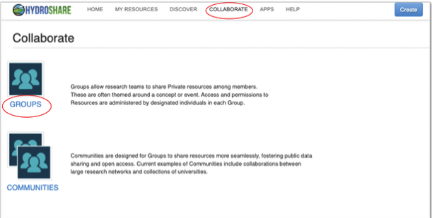
The “Find Groups” page can then be used to find a listing of discoverable and public groups available. Using the search function users can enter keywords which may be associated with group names, purpose, descriptions and other keywords indexed by the group owner.

Discover the HI-DSI Group
Use HydroShare’s search functionality to find the HydroShare group named, “HI-DSI Gateways and Workflows”.
Click on the title of any listed group to view the groups landing page. Members of public groups can be seen by searching users while the members of a discoverable group can not be seen. Either way users can request group membership.
Joining a Group
Once a group of interest is found, users can request access by clicking the “Ask to join” button. If the owner of the group has not set the “auto accept” option for new requests, users may experience a wait time until their request is processed. Otherwise, access may be granted almost immediately.
Join the HI-DSI Group
Once the “HI-DSI Gateways and Workflows” group is found, request access by clicking, “Ask to join”.
About Groups
A groups landing page will provide some information about the group such as the groups title, purpose and description of the group. From the landing page, users will be able to see all resources shared with the group as well as all members of the group. It should be noted that resources within the group are not owned by all members. While they are shared, ownership is retained by the individual user which created the resource.
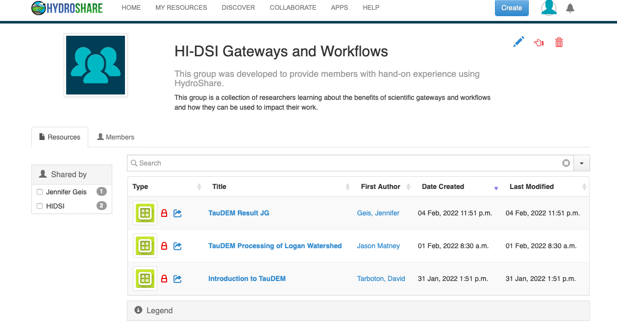
Exercise: Using Resources and Workflows Within a Group to Collaborate On Data Analysis
For this exercise, attendees who have joined the HI-DSI group will use an existing shared resource containing both data and a Jupyter Notebook workflow to perform some visualization and data analysis. The purpose of this exercise is to:
- Demonstrate how a gateway can provide a collaborative environment
- Demonstrate how data workflows can ease the researchers burden of programming certain computational tasks from scratch.
- Exemplify the usefulness of gateways and workflows in the reproducibility of scientific results.
HydroShare supports various web apps which workflows and models can be built in. Typically, most hydrological modeling and data analysis is done on a personal computer or on some centralized computing system. A user’s knowledge of such centralized computing system could all be barriers to the user’s research. Some examples could be:
- Knowledge about high-performance computing systems
- Capacity of a local computer
- Compatability and dependency requirements for installation on local computers, and
- Time taken to get local model installations properly configured and validated
By providing and supporting web apps such as JupyterHub and its Jupyter Notebook functionality, HydroShare enables a more flexible environment for model execution and data analysis. This gives users a preconfigured environment free of worry about cyberinfrastructure and dependencies thus lowering the forementioned barriers to research.
A Jupyter notebook contains live code, equations, visualization, and explanatory text. They can be used to implement scientific workflows and other computational tasks. HydroShare users can either create and share their own workflows using Jupyter notebooks or discover and use existing workflows implemented as Jupyter notebooks.
Jupyter Notebook functionality within HydroShare:
- Notebooks can be launched from HydroShare
- Notebooks can access the contents of HydroShare resources
- Notebooks can save results back into HydroShare
Ease of Use For the User
The code within a Jupyter notebook can execute operating and language specific commands within the hosting environment. This provides users with access to the hosting environment’s computational capabilities while eliminating the need for users to install and configure software.
While this does not relieve the user from needing to learn the programming language, operating system commands, or commands associated with the program being used for analysis, it does remove the need for users to install and have the capacity to run these programs locally.
About the Following Exercise
For this exercise attendees will be performing some visualization and data analysis on a raw .tif file of a geographic region. They will use an existing workflow to perform some common computational tasks on the type of data provided using a software package for digital elevation models called TauDEM. Attendees will then perform further analysis on the data and write their results back to HydroShare as a new separate resource. This resource can then be shared with a group for further scientific collaboration.
The Data
The data used will be a single image. The file was raster data of a surface map and was saved in a .tif format. It is an aerial image of a mountain and water source in Utah.
Rasters are well suited for representing data that changes continuouosly across a surface landscape. They provide an effective method of storing the continuity as a surface. Elevation values measured from the Earth’s surface are the most common application of surface maps.
About TauDem:
Terrain Analysis Using Digital Elevation Models (TauDEM) is a software for Hydrologic Terrain Analysis in Jupyter. TauDEM is a free and open source set of Digital Elevation Model (DEM) tools for the extraction and analysis of hydrologic information from topography as represented by DEM. This software is developed at Utah State University (USU) for hydrologic digital elevation model analysis and watershed delineation.
Further information on the use of TauDEM functions can be found in the TauDEM documentation
Workflows and the TauDEM Notebook
Existing workflows can be helpful in that they remove the need for a researcher to program some common computational tasks for their data from scratch. The idea behind using the TauDEM notebook for this exercise is to use the existing workflow set in place to perform some data analysis and visualization. Users can then perform further analyses to meet their needs. This exemplifies the collaboration aspect which a gateway can provide its users.
Users will use an existing workflow developed by David Tarboton, Director of Utah Water Research Laboratory, in order to run some commonly used visualization and computational methods on digital elevation models. The goal will be to perform some additional analysis in Professor Tarboton’s notebook in order to delineate a subwatershed and a stream network using some given TauDem functions. User’s will then write the Jupyter Notebook with their additional analysis into a new HydroShare resource which can then be shared with their research group.
Workflow for Terrain Analysis Using Digital Elevation Models
To make it easier to follow along with the hands-on portion of this workshop and to understand what each individual cell in the Jupyter Notebook is doing we will break every task into “Steps”.
Step 1: Accessing the JupyterHub Notebook
- Once on the group landing page, select the resource titled “HI-DSI Workshop: Introduction to TauDEM”
- Click “Open with” at the top right.
- Choose CUAHSI JupyterHub as the webapp.
- Agree to the terms of use and click “Sign in with HydroShare”.
- Authorize CUAHSI JupyterHub. The JupyterHub session will open.
- Select the Python environment ‘Python - v3.8’
- Select the file at the top of the list named WorkshopTauDEM.ipynb.
Step 2: Install and Import Libraries
Note that Professor Tarboton’s comments are included in the notebook to help users find documentation and understand what task each cell performs.
The first cell in the notebook is like most Jupyter Notebooks. All necessary software are installed in the users’ JupyterHub using the pip command. Module imports are also carried out here. The hstools module provides functions for interacting with HydroShare, including resource querying, downloading and creation. The TauDEM module provides functions for workspace maintenance, data analysis as well as visualization.
# Only run this cell if the libraries are not already installed
!pip install rasterio
!pip install geopandas
!pip install hstools


import os
import rasterio as rio
%matplotlib inline
from matplotlib import pyplot as plt
from matplotlib import colors

! pwd

! ls
Step 3: Define a Plotting Function For Visualization
We start with a digital elevation model, DEM, file surrounding the Logan River Watershed in Logan, Utah. The file is named logan.tif. In this section, we illustrate the TauDEM basic grid analysis functions. TauDEM uses files in TIFF format by default.
This workflow first defines a visualization function which can be repeatedly used in order to plot data and resulting figures after analysis. The function is already defined for the user. It can be called on the data file to visualize.
Defining a convenient plotting function
# Define convenience plotting function
cmap='terrain'
label='Elevation (m)'
import math
import numpy as np
def rp(raster,cmap='terrain',label='',bounds=[]):
    with rio.open(raster) as src:
        boundary = src.bounds
        parray = src.read()
        nodata = src.nodata
        parray=np.where(parray == nodata,math.nan,parray)

    # Plot the imported data
    plt.figure(figsize=(20,10))
    # if using bounds
    if(len(bounds) > 0):
        bounds=np.insert(bounds,0,np.nanmin(parray))
        bounds=np.append(bounds,np.nanmax(parray))
        norm = colors.BoundaryNorm(bounds, cmap.N)
        imgplot = plt.imshow(parray[0],cmap=cmap,norm=norm)
    else:
        imgplot = plt.imshow(parray[0],cmap=cmap)
    cbar = plt.colorbar()
    cbar.set_label(label)
    # plt.savefig('LoganDEM.png', dpi=450, bbox_inches = 'tight')   # activate this command if you want to save the figure. Note that it should be called before plt.show()
    plt.show()
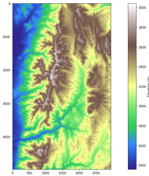
Calling the function on the data provides a visualization of the original file.
# display the raw dem
dem = 'logan.tif'
rp(dem,label="Elevation (m)",)
Step 4: Removing Pits From Data
Next, this workflow begins grid analysis by calling actual TauDEM functions; the first of which is Pit Remove. Pits are grid cells surrounded by higher terrain that do not drain. It is important to remove these pits in order that a more hydrologically conditioned image is created from the original for further analysis. Pits are removed by raising the elevation of pits.
The output of this function will provide information on how long execution might take along with some other system and file information.
!mpiexec -n 4 pitremove {dem}
After execution is done there will be an additional file which is a hydrologically conditioned DEM as previously mentioned.
! ls  # This lists the files present.
# Note you should see the additional output file loganfel.tif that was written by the previous command.

loganfel.tif	  logan.tif   Outlet_meta.xml	 Outlet.shp
logan_meta.xml	  logan.vrt   Outlet.prj	 Outlet.shx
logan_resmap.xml  Outlet.dbf  Outlet_resmap.xml  TauDEM.ipynb
Step 5: D8 Analysis
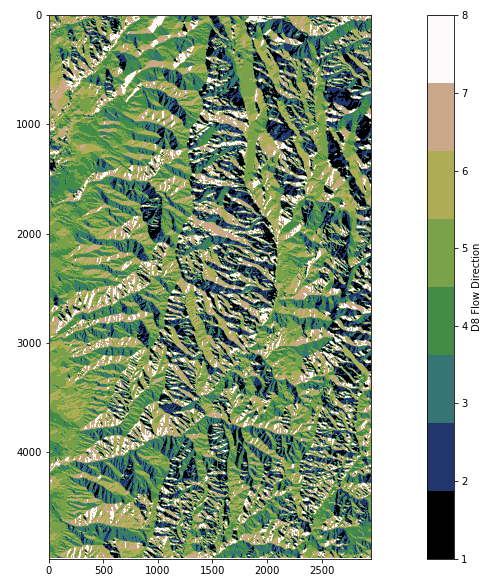
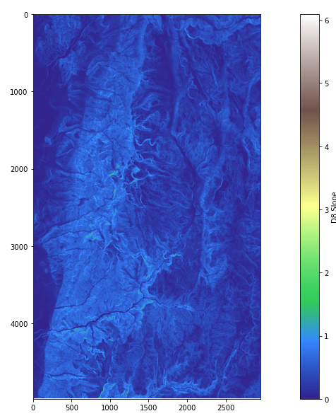
The conditioned file with pits removed is then used to perform a D8 analysis. D8 analysis calculates the directions of flow from each cell to its downslope neighbor or neighbors using the D8, D-Infinity (DINF), or Multiple Flow Direction (MFD) method. The TauDEM function used is called d8flowdir and it will output two new files named loganp.tif and logansd8.tif.
Once executed, the function takes a few minutes to complete calculations and produce output files.
!mpiexec -n 4 d8flowdir -p loganp.tif -sd8 logansd8.tif -fel loganfel.tif
Calling the previously defined plotting function, the resulting files, loganp.tif and logansd8.tif, can be visualized.
rp('loganp.tif',plt.get_cmap('gist_earth', 8),'D8 Flow Direction')
rp('logansd8.tif','terrain','D8 Slope')
Step 6: Stream Drop Analysis
The next cell runs a sequence of TauDEM functions to identify the optimal threshold to use to delineate the stream network. The analysis uses TauDEM’s stream drop analysis approach which is based on the weighted contributing area of upward curved grid cells which are mapped using the Peuker Douglas algorithm.
The corresponding output file will be Outlet.shp.
The last command in the sequence, “drop analysis”, maps the highest resolution stream network consistent with the DEM’s geographic morphology and determines the drainage density. It does this by testing a number of stream delineation thresholds. It identifies the threshold where the mean stream drop for first order streams is not statistically different from the mean stream drop of higher order streams.
Execution of these commands will take a few minutes and output some runtime information.
!mpiexec -n 4 aread8 -p loganp.tif -o Outlet.shp -ad8 loganad8o.tif
!mpiexec -n 8 peukerdouglas -fel loganfel.tif -ss loganss.tif -par 0.4 0.1 0.05
!mpiexec -n 8 aread8 -p loganp.tif -ad8 loganssa.tif -wg loganss.tif -o Outlet.shp
!mpiexec -n 8 dropanalysis -fel loganfel.tif -p loganp.tif -ad8 loganad8o.tif -ssa loganssa.tif -o Outlet.shp -drp logandrp.txt -par 10   1000 15 0

# Determine threshold from last line of drp.txt file after colon.
with open("logandrp.txt", 'r') as f:
    lines = f.read().splitlines()
thresh=lines[len(lines)-1].split(":")[1]
print("\nOptimal stream definition threshold:"+thresh)
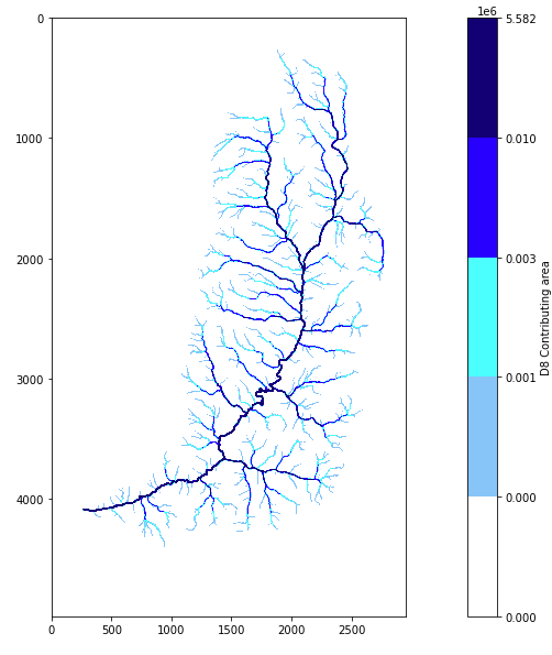
Plot the results using the defined visualization function. The following is the high resolution stream network and portions of the network which contribute more flow within the watershed. This will serve to perform further analysis of the stream network using TauDEM.
rp('loganad8o.tif',colors.ListedColormap(['white', 'lightskyblue', 'cyan', 'blue', 'navy']),'D8 Contributing area',bounds=[300,1000,3000,10000])
Step 7: Stream Network Analysis Using TauDEM functions
In the following steps, users will perform their own analysis to add to this workflow. Since workshop attendees are not expected to be familiar with hydro-sciences or TauDEM, some code will be provided to perform further analysis on the stream network obtained using Professor Tarboton’s workflow. Attendees are encouraged to follow along by copying the provided code here into the Jupyter Notebook in the group resource. They will then be able to save their additions as a new resource into HydroShare using given HydroShare tool commands.
Keep in mind that the important point of this exercise is to experience the collaborative nature scientific gateways can provide. Also the benefit scientific workflows bring to researcher’s work by providing code for common data analysis tasks.
Our goal will be to delineate a watershed and the parts of the stream network which contribute most to water flow.
Using the extracted high resolution stream network, we will use the TauDEM function “threshold” to define a stream raster grid named logansrc.tif. The threshold function uses as input the previously obtained file named loganssa.tif which is a weighted contributing area or the stream source accumulation, ssa, and the threshold determined using the “drop analysis” function.
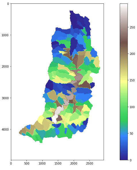
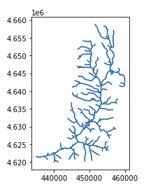
The “streamnet” function will provide a number of output files including the target files of interest. Outputs will include the shapefile named logannet.shp which will be the portion of the stream network consisting of most water flow and a shapefile with delineated subwatersheds named loganw.tif. This data file represents the amount each portion of the watershed drains to each link of the stream network.
Inputs to these functions include outputs from previous analysis in Professor Tarboton’s workflow.
!mpiexec -n 4 threshold -ssa loganssa.tif -src logansrc.tif -thresh {thresh}
!mpiexec -n 4 streamnet -fel loganfel.tif -p loganp.tif -ad8 loganad8o.tif -src logansrc.tif -ord loganord3.tif -tree logantree.dat -coord logancoord.dat -net logannet.shp -w loganw.tif -o Outlet.shp
Using the plotting function to visualize the delineated watershed.
rp('loganw.tif')
Any resulting output files produced through further analysis will be written to the working directory within JupyterHub and ultimately into the resource written back to HydroShare.
The following list of files are all the output files produced from previous analysis. These will all be saved and stored into a new HydroShare resource.
!ls
loganad8o.tif	logannet.shp	  loganssa.tif	 Outlet_meta.xml
logancoord.dat	logannet.shx	  loganss.tif	 Outlet.prj
logandrp.txt	loganord3.tif	  logan.tif	 Outlet_resmap.xml
loganfel.tif	loganp.tif	  logantree.dat  Outlet.shp
logan_meta.xml	logan_resmap.xml  logan.vrt	 Outlet.shx
logannet.dbf	logansd8.tif	  loganw.tif	 TauDEM.ipynb
logannet.prj	logansrc.tif	  Outlet.dbf
The “geopandas” library is used to visualize the stream network shapefile. The following code imports those libraries, reads the file and plots the resulting stream network.
When importing geopandas there will be a compatibiliy warning. This won’t be a problem and the cell will still run.
from geopandas import GeoSeries, GeoDataFrame, read_file, gpd

streamnet = read_file('logannet.shp')
streamnet

plt.figure(figsize=(30, 24))
streamnet.plot()
Congratulations
Congratulations! You have successfully delineated subwatersheds and a stream network using TauDEM. If you want to retain your work you could at this point save the contents of your folder back to HydroShare, or download them.
Step 8: Save the Results Back To HydroShare
Note about HydroShare tools
Recall that Jupyterhub communicates with HydroShare via the Hydroshare REST API. CUAHSI has provided a set of utilities which serve as a means to communicate with HydroSHare from within JupyterHub. These tools can be installed from within the Jupyter notebook using the command ‘!pip install hstools’.
When installed, more information on how to use hstools can be found by executing the command ‘!hs –help’.
!hs --help

usage: hs {get, add, create, delete, list, describe, init} [-h, --help]

HSTools is a humble collection of tools for interacting with data in the
HydroShare repository. It wraps the HydroShare REST API to provide simple
commands for working with resources.

positional arguments:
  {get,add,create,delete,list,describe,init}
    get                 Retrieve resource content from HydroShare
    add                 Add files to an existing HydroShare resource
    create              Create a new HydroShare resource
    delete              Delete a HydroShare resource
    list                List HydroShare resources that you own
    describe            Describe metadata and files
    init                Initialize a connection with HydroShare

optional arguments:
  -h, --help            show this help message and exit
The HydroShare “hstools” library will be used to save the changes and additions made to the Jupyter notebook in this exercise back to HydroShare as a new resource. A new HydroShare resource can be created using the ‘!hs create’ command in a separate notebook cell. The ‘!hs create –help’ command provides information on how to use the command.
!hs create --help
usage: hs create  [-q] [-v] [-f] [-k] [-t] [-a] [-h]

Create a new HydroShare resource

optional arguments:
  -h, --help            show this help message and exit
  -a ABSTRACT [ABSTRACT ...], --abstract ABSTRACT [ABSTRACT ...]
                    resource description
  -t TITLE [TITLE ...], --title TITLE [TITLE ...]
                    resource title
  -k KEYWORDS [KEYWORDS ...], --keywords KEYWORDS [KEYWORDS ...]
                    space separated list of keywords
  -f FILES [FILES ...], --files FILES [FILES ...]
                    space separated list of files
  -v                    verbose output
  -q                    suppress output
Before creating the resource, a few notes should be mentioned. First, metadata can be defined within JupyterHub using Python lists and strings. In order to create a resource, certain metadata fields must be included. These fields are the title, abstract, keywords, and content files. It is also important to know and include the files intended to be written to the HydroShare resource.
Users can view all of the files in their directory using the ‘!ls’ command before selecting which to write back to HydroShare as part of the new resource.
!ls
loganad8o.tif	logannet.shp	  loganssa.tif	 Outlet_meta.xml
logancoord.dat	logannet.shx	  loganss.tif	 Outlet.prj
logandrp.txt	loganord3.tif	  logan.tif	 Outlet_resmap.xml
loganfel.tif	loganp.tif	  logantree.dat  Outlet.shp
logan_meta.xml	logan_resmap.xml  logan.vrt	 Outlet.shx
logannet.dbf	logansd8.tif	  loganw.tif	 TauDEM.ipynb
logannet.prj	logansrc.tif	  Outlet.dbf
The following code block defines all required metadata for resource creation.
# define metadata variables

keywords = ['TauDEM', 'Logan River']
abstract = "Jupyter Notebook TauDEM was used to define streamflow and subwatersheds in the Logan River Watershed in Utah."

title = "Test TauDEM Result"
files = !find . -maxdepth 1 -type f     # shows all the files created
print(files)

# Select the files that you want to save
files = ['./logan.tif', './TauDEM.ipynb',
        'Outlet.shp','Outlet.prj',
        'Outlet.shx','Outlet.dbf'
]
The following code block is used to initialize HydroShare. It provides authorization from the current location within JupyterHub to write into HydroShare. Users will be asked to sign into HydroShare to connect and write their resource.
It should be noted that according to the ‘hstools’ library, the ‘!hs init’ command can be used to initialize a connection with HydroShare, however there seemed to be an issue using it in conjuction with this notebook. Professor Tarboton provided this block of code in which he defined his own intialization function which was used here. Users are encouraged to try the HydroShare utilities function ‘!hs init’ in their own project when writing back to HydroShare.
# Initialize HydroShare connection
# This is an awkward way to initialize the HydroShare connection from inside Jupyter.  An alternative is to open
# a terminal and run hs init
import hstools as hs
import os
import sys
import json
import base64
import argparse
from getpass import getpass
from hstools import hydroshare
def init(loc='.'):
    fp = os.path.abspath(os.path.join(loc, '.hs_auth'))
    if os.path.exists(fp):
        print(f'Auth already exists: {fp}')
        remove = input('Do you want to replace it [Y/n]')
        if remove.lower() == 'n':
            sys.exit(0)
        os.remove(fp)

    usr = input('Enter HydroShare Username: ')
    pwd = getpass('Enter HydroShare Password: ')

    dat = {'usr': usr,
          'pwd': pwd}
    cred_json_string = str.encode(json.dumps(dat))
    cred_encoded = base64.b64encode(cred_json_string)
    with open(fp, 'w') as f:
        f.write(cred_encoded.decode('utf-8'))

    try:
        hydroshare.hydroshare(authfile=fp)
    except Exception:
        print('Authentication Failed')
        os.remove(fp)
        sys.exit(1)

    print(f'Auth saved to: {fp}')
init('/home/jovyan')
Finally, create the new resource in Hydroshare using the ‘!hs create’ command. After executing, the command output will provide a link to the HydroShare resource. Users can access the resource directly by clicking on the link or by using the “My Resources” tab in the HydroShare website.
!hs create -t {title} -a {abstract} -k {' '.join(keywords)} -f {' '.join(files)}
+ creating resource
+ adding: ./logan.tif
+ adding: ./TauDEM.ipynb
+ adding: Outlet.shp
+ adding: Outlet.prj
+ adding: Outlet.shx
+ adding: Outlet.dbf
After executing, the command output will provide a link to the HydroShare resource. Users can access the resource directly by clicking on the link or by using the “My Resources” tab in the HydroShare website. Click on the new resource and use the share button share the new resource with the “HI-DSI Scientific Gateways and Workflows” group. Other group members are now able to access the new resource and view the methods used in your analysis and further add to it or use it for the own data analysis and research.
This exercise was meant to emphasize how scientific gateways and workflows can help researchers collaborate, reproduce science, get started quickly with some data related tasks, and help satisfy data management plans.
Key Points
Scienctific gateways like HydroShare, enable researchers to form and join groups and communities, within the gateway, with similar research interests.
Existing workflows can be discovered and used to aid researchers perform visualization and analysis on their data, eliminating the need to write all the necessary foundational codes.